<video width="420" controls>
  <source src="mov_bbb.mp4" type="video/mp4">
  <source src="mov_bbb.ogg" type="video/ogg">
 Your browser does not support the video tag.
</video>ENV222 NOTE
R in statistics (Advanced)
Hyperlink of XJTLU ENV222 courseware
- Lecture-1 ENV222 Overview
- Lecture-2 R Markdown basic
- Lecture-3 R Markdown advanced
- Lecture-4 R for characters
- Lecture-5 R for time data
- Lecture-6 Statistical graphs (advanced)
- Lecture-7 R Tidyverse
- Lecture-8 ANOVA Post-hoc tests
- Lecture-9 MANOVA
- Lecture-10 ANCOVA
- Lecture-11 MANCOVA
- Lecture-12 Combining statistics
- Lecture-13 Non-parametric hypothesis tests
- Lecture-14 Multiple linear regression
- Lecture-15 Logistic regression
- Lecture-16 Poisson regression
- Lecture-17 Non-linear regression
- Lecture-18 Tests for distributions
- Lecture-19 Principal component analysis
- Lecture-20 Cluster analysis
The meaning of each parameter in statistical table (Chinese)
- Df(自由度): 回归自由度(regression degrees of freedom)和误差自由度(error degrees of freedom)的总数,其中回归自由度为解释变量的个数减1,误差自由度为样本量减去解释变量的个数。
- Sum Sq(平方和): 每个来源的平方和(sum of squares),是变量离均差的平方和。回归平方和(regression sum of squares)表示自变量对因变量的影响程度,误差平方和(error sum of squares)表示自变量未能解释的部分。
- Mean Sq(均方): 每个来源的均方(mean square),是平方和除以自由度得到的平均数。回归均方(regression mean square)表示每个自变量对因变量的影响程度,误差均方(error mean square)表示自变量未能解释的部分的平均方差。
- F value: 回归均方与误差均方的比值,用于判断模型的拟合程度,F值越大则模型越好。在一元线性回归中,F值等于t值的平方。
- Pr(>F): Probability of obtaining a larger F value(得到更大的F值的概率)Pr(>F)是F检验得到的P值。p值越小则说明结果越显著,一般将显著性水平设为0.05,即当p值小于0.05时认为结果具有统计显著性。
- Pillai: Pillai trace(皮莱迹)是在多元方差分析中使用的一种统计量,用于衡量所有因素对因变量的共同影响程度。
- approx F: F approximation(F近似值)是根据Pillai迹值计算出来的F值。它用于评估多元方差分析的总体显著性。
- num Df: Numerator degrees of freedom(分子自由度)指的是分子中的自由度。
- den Df: Denominator degrees of freedom(分母自由度)指的是分母中的自由度。
- Residuals: 残差,是指多元方差分析中的误差项,即不能被自变量解释的因变量方差。
- Intercept: 截距,也称为常数项,表示当自变量为0时,因变量的预测值(或期望值)。
- Estimate: 回归系数,表示自变量每增加一个单位时,因变量发生的平均变化量。
- Std.Error: 标准误差,表示估计值的不确定性或误差,即估计值与真实值之间的平均差异。
- t value: t值,表示回归系数的显著性,即回归系数除以其标准误差,得到的值与t分布相比较的结果。
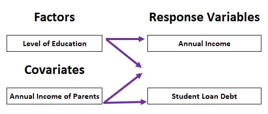
How to choose between ANOVA, MANOVA, ANCOVA and MANCOVA (Chinese)
ANOVA、MANOVA、ANCOVA和MANCOVA都是统计学中常见的分析方法,主要用于比较两个或多个组之间的差异性,并用统计学方法对这些差异进行推断和验证。
- ANOVA(Analysis of Variance):方差分析,用于比较两个或多个组的均值是否有显著差异,适用于只有一个自变量和一个因变量的情况。例如,用于比较不同教学方法对学生成绩的影响是否有显著差异。
- MANOVA(Multivariate Analysis of Variance):多元方差分析,用于比较两个或多个组的多个相关因变量是否有显著差异,适用于有多个相关因变量的情况。例如,用于比较不同教学方法对学生成绩、学生态度和学生动机等多个方面的影响是否有显著差异。
- ANCOVA(Analysis of Covariance):协方差分析,用于比较两个或多个组的均值是否有显著差异,并控制一个或多个协变量(即影响因素),适用于需要控制其他因素影响的情况。例如,用于比较不同教学方法对学生成绩的影响是否有显著差异,同时控制学生的初始水平,避免学生初始水平的不同对比较结果产生影响。
- MANCOVA(Multivariate Analysis of Covariance):多元协方差分析,同时控制多个协变量,比较两个或多个组的多个相关因变量是否有显著差异,适用于有多个相关因变量和多个协变量的情况。例如,用于比较不同教学方法对学生成绩、学生态度和学生动机等多个方面的影响是否有显著差异,同时控制学生的初始水平、性别、年龄等因素的影响。
👉🏻Click to enter the ENV222 exercise section
👉🏻Click to enter the ENV221 note section
1 R-markdown(qmd, html) syntax
1.1 Fundamental
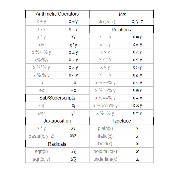
Subscript by Rmarkdown: Use
PM~2.5~to form PM2.5.
Subscript by html:log<sub>2</sub>will be displayed as log2.Superscript by Rmarkdown: Use
R^2^to form R2.
Superscript by html:2<sup>n</sup>will be displayed as 2n.Use
$E = mc^2$to form \(E = mc^2\)Use
[Link of XJTLU](http://xjtlu.edu.cn)to form Link of XJTLUUse
<mark>text</mark>to highlight the textUse
<u>text</u>to add underline to the textUse
<center><img src="images/rstudio-qmd-how-it-works.png" width="1400" height="257"/>or<center> {width=100%}to form
Rstudio qmd how it works Use
<iframe src="https://www.r-project.org/" width="100%" height="300px"></iframe>to form a windows which show another file on-line, like this:Use the following HTML code to add a video to your Rmarkdown(HTML):
Use something like
{r, fig.width = 6, fig.height = 4, fig.align='center'}in front of the code chunk to change the output graphicsAlso, use
{r, XXX-Plot, fig.cap="XXX-Plot"}in the front of code chunk to add a caption of this figureUse something like
<span style="color:red; font-weight:bold; font-size:16px; font-family:Tahoma;">sentence</span>to change the properties of textWhen we need to post some statistic analysis and formula in Rmarkdown we can use these code template below (fill
datain):
# Equation
equatiomatic::extract_eq(data, use_coefs = TRUE)
# Analysis
stargazer::stargazer(data, type = 'text')- Use the following HTML code to add a foldable item to your Rmarkdown(HTML):
<details>
  <summary>title</summary>
  content
</details>
title
content- Use
| Name | Math | English |
|:----:|:-----|--------:|
| Tom | 93 | 100 |
| Mary | 60 | 90 |
to form
| Name | Math | English |
|---|---|---|
| Tom | 93 | 100 |
| Mary | 60 | 90 |
- Or use
library(knitr)
df <- data.frame(
  Math = c(80, 90),
  English = c(85, 95),
  row.names = c("Tom", "Mary")
)
kable(df, format = "markdown")| Math | English | |
|---|---|---|
| Tom | 80 | 85 |
| Mary | 90 | 95 |
- Use
- 1.
- 2.
    - 1.
    - 2.
- 3.
to form sub-rank like this below:
1.2 Advanced
- Numbering, caption, and cross-reference of R-plots in academic paper Click to see the detail in ENV222 Week5-5.2
2 Basic R charaters
2.1 Check the data type
# import dataset
x <- 'The world is on the verge of being flipped topsy-turvy.'
dtf <- read.csv('data/student_names.csv')
head(dtf)
Name Prgrm
1 Yuzhou Liu Bio
2 Penghui Wang Bio
3 Ziang Li Eco
4 Youcheng Jin Bio
5 Yuge Yang Bio
6 Yutian Song Eco# data type
class(x)[1] "character"# length of the dataset
length(x)[1] 1# length of the sub dataset
nchar(x)[1] 552.2 Index to maximum and minimum values
- Find the longest name in student_names.csv,
which.maxorwhich.minis used to find the index of the (first) minimum or maximum of a numeric (or logical) vector
name_n <- nchar(dtf$Name)
name_nmax <- which.max(name_n)
dtf$Name[name_nmax]
[1] "Iyan Hafiz Bin Mohamed Faizel"# or
dtf$Name[which.max(nchar((dtf$Name)))][1] "Iyan Hafiz Bin Mohamed Faizel"# or
library(magrittr)
dtf$Name %>% nchar() %>% which.max() %>% dtf$Name[.][1] "Iyan Hafiz Bin Mohamed Faizel"2.3 Capital and small letter
# tolower() toupper()
(xupper <- toupper(x))
[1] "THE WORLD IS ON THE VERGE OF BEING FLIPPED TOPSY-TURVY."(dtf$pro <- tolower(dtf$Prgrm)) [1] "bio" "bio" "eco" "bio" "bio" "eco" "bio" "bio" "eco" "bio" "eco" "bio"
[13] "bio" "env" "bio" "bio" "bio" "env" "bio" "env" "bio" "bio" "bio" "bio"
[25] "eco" "eco" "env" "bio" "bio" "bio" "bio" "env" "bio" "bio" "bio" "bio"
[37] "bio" "eco" "eco" "bio" "bio" "bio" "bio" "bio" "bio" "bio" "bio" "eco"
[49] "bio" "bio" "env" "eco" "eco" "bio" "env" "env" "env"2.4 Split string
# strsplit()
x_word <- strsplit(xupper, ' ')
class(x_word)
[1] "list"# If you want to extract the first element in the list, you need to use double brackets [[]], and if you want to extract the first sublist in the list, use single brackets []
x_word1 <- x_word[[1]]
class(x_word1)[1] "character"table(x_word1) # Form a table which involved the frequency of each char acterx_word1
BEING FLIPPED IS OF ON THE
1 1 1 1 1 2
TOPSY-TURVY. VERGE WORLD
1 1 1 x_word1[!duplicated(x_word1)] # Find the distinct characters in the list by use duplicated() function[1] "THE" "WORLD" "IS" "ON" "VERGE"
[6] "OF" "BEING" "FLIPPED" "TOPSY-TURVY."unique(x_word1) # Other way yo detect the distinct characters[1] "THE" "WORLD" "IS" "ON" "VERGE"
[6] "OF" "BEING" "FLIPPED" "TOPSY-TURVY."lapply(x_word, length) # The output of the lapply() function is a list[[1]]
[1] 10sapply(x_word, length) # The output of the sapply() function is a vector or a matrix[1] 10sapply(x_word, nchar) [,1]
[1,] 3
[2,] 5
[3,] 2
[4,] 2
[5,] 3
[6,] 5
[7,] 2
[8,] 5
[9,] 7
[10,] 122.5 Separate column
# separate() is a function in the tidyr package that can be used to split a column in a data box into multiple columns
library(tidyr)
dtf2 <- separate(dtf, Name, c("GivenName", "LastName"), sep = ' ')  # separate(data, col, into, sep)
dtf$FamilyName <- dtf2$LastName
head(dtf)
Name Prgrm pro FamilyName
1 Yuzhou Liu Bio bio Liu
2 Penghui Wang Bio bio Wang
3 Ziang Li Eco eco Li
4 Youcheng Jin Bio bio Jin
5 Yuge Yang Bio bio Yang
6 Yutian Song Eco eco Song2.6 Extract
The world is on the verge of being flipped topsy-turvy.
# substr() is a built-in function in R that can be used to extract or replace substrings from a character vector
substr(x, 13, 15)  # substr(x, start, stop)
[1] " on"dtf$NameAbb <- substr(dtf$Name, 1, 1)
head(dtf, 3) Name Prgrm pro FamilyName NameAbb
1 Yuzhou Liu Bio bio Liu Y
2 Penghui Wang Bio bio Wang P
3 Ziang Li Eco eco Li Z2.7 Connect
# paste() function can convert multiple objects into character vectors and concatenate them
paste(x, '<end>', sep = ' ')  # paste(x1, x2,... sep, collapse)
[1] "The world is on the verge of being flipped topsy-turvy. <end>"paste(dtf$NameAbb, '.', sep = '') [1] "Y." "P." "Z." "Y." "Y." "Y." "H." "A." "E." "J." "Y." "M." "Y." "Y." "X."
[16] "Z." "W." "J." "Q." "Y." "F." "Y." "Z." "M." "Z." "S." "X." "J." "R." "Z."
[31] "Y." "X." "Z." "Y." "Q." "Y." "Y." "M." "Q." "J." "Y." "X." "M." "Q." "Y."
[46] "P." "Y." "J." "L." "Y." "Q." "H." "Z." "H." "J." "Y." "I."paste(dtf$NameAbb, collapse = ' ') # collapse = ' ' put all of the characters into a character[1] "Y P Z Y Y Y H A E J Y M Y Y X Z W J Q Y F Y Z M Z S X J R Z Y X Z Y Q Y Y M Q J Y X M Q Y P Y J L Y Q H Z H J Y I"paste(dtf$NameAbb, dtf$FamilyName, sep = '. ')[7] # This is my name for academic essay cite[1] "H. Zhu"2.8 Find
# grep() function in R is a built-in function that searches for a pattern match in each element of character
y <- c("R", "Python", "Java")
grep("Java", y)
[1] 3for(i in 1:length(y)) {
print(grep(as.character(y[i]), y))
}[1] 1
[1] 2
[1] 3sapply(y, function(x) grep(x, y)) R Python Java
1 2 3 head(table(dtf2$GivenName), 12)
      Adriel        Elina       Fengyi        Haode       Hongli Huangtianchi
           1            1            1            1            1            1
        Iyan       Jiajie       Jiawei        Jiayi      Jingyun       Jiumei
1 1 1 2 1 1 grep('Jiayi', dtf$Name, value = TRUE)[1] "Jiayi Chen" "Jiayi Guo" grep('Jiayi|Guo', dtf$Name, value = TRUE)[1] "Jiayi Chen" "Fengyi Guo" "Jiayi Guo" # regexpr() function is used to identify the position of the pattern in the character vector, where each element is searched separately.
z <- c("R is fun", "R is cool", "R is awesome")
regexpr("is", z) # Returns include starting position, duration length, data type ...[1] 3 3 3
attr(,"match.length")
[1] 2 2 2
attr(,"index.type")
[1] "chars"
attr(,"useBytes")
[1] TRUEgregexpr("is", z) # The gregexpr() function returns all matching positions and lengths, as a list[[1]]
[1] 3
attr(,"match.length")
[1] 2
attr(,"index.type")
[1] "chars"
attr(,"useBytes")
[1] TRUE
[[2]]
[1] 3
attr(,"match.length")
[1] 2
attr(,"index.type")
[1] "chars"
attr(,"useBytes")
[1] TRUE
[[3]]
[1] 3
attr(,"match.length")
[1] 2
attr(,"index.type")
[1] "chars"
attr(,"useBytes")
[1] TRUE2.9 Replace
# gsub()
gsub(' ', '-', x)
[1] "The-world-is-on-the-verge-of-being-flipped-topsy-turvy."2.10 Regular expression
# help(regex)
# Find the one who has a given name with 4 letters and a family name with 4 letters
grep('^[[:alpha:]]{4} [[:alpha:]]{4}$', dtf$Name, value = TRUE)
[1] "Yuge Yang" "Ziyu Yuan" "Qian Chen" "Ying Zhou"# Here, parentheses are used to create a capturing group. A capturing group is a subexpression of a regular expression that can capture and store the matched text during matching.
# In this example, the capturing group is used to extract the first word from the string. Without a capturing group, the entire matched string would be replaced with \\1 instead of just the first word.
dtf$FirstName <- gsub('^([^ ]+).+[^ ]+$', '\\1', dtf$Name)
head(dtf) Name Prgrm pro FamilyName NameAbb FirstName
1 Yuzhou Liu Bio bio Liu Y Yuzhou
2 Penghui Wang Bio bio Wang P Penghui
3 Ziang Li Eco eco Li Z Ziang
4 Youcheng Jin Bio bio Jin Y Youcheng
5 Yuge Yang Bio bio Yang Y Yuge
6 Yutian Song Eco eco Song Y YutianRmarkdown 中正则表达式的基本语法如下:
. 匹配任意单个字符,除了换行符。
[ ] 匹配方括号内的任意一个字符,例如 [abc] 匹配 a 或 b 或 c。
[^ ] 匹配方括号外的任意一个字符,例如 [^abc] 匹配除了 a 和 b 和 c 之外的任意字符。
- 在方括号内表示范围,例如 [a-z] 匹配小写字母, [0-9] 匹配数字。
\d \D \w \W \s \S 分别匹配数字、非数字、单词字符(字母、数字和下划线)、非单词字符、空白符(空格、制表符和换行符)、非空白符。
\b \B ^ $ \ 分别匹配单词边界(单词和非单词之间)、非单词边界(两个单词或两个非单词之间)、字符串开头、字符串结尾、转义符(用于匹配元字符本身)。
( ) | ? + * { } \ 分别匹配分组或捕获子表达式(可以用反斜杠加数字引用),选择(匹配左边或右边),零次或一次重复,一次或多次重复,零次或多次重复,指定重复次数,零宽断言(匹配位置而不是字符)。
简单的例子,查找 Markdown 链接([This is a link](https://www.example.com)):
\[([^\]]+)\]\(([^)]+)\)
这个正则表达式可以分解为以下部分:
\[ 匹配左方括号
([^\]]+) 匹配并捕获一个或多个不是右方括号的字符
\] 匹配右方括号
\( 匹配左圆括号
([^)]+) 匹配并捕获一个或多个不是右圆括号的字符
\) 匹配右圆括号3 Time data in R
3.1 Format of time
# Check the current date
date()
[1] "Mon May 22 15:43:52 2023"# character
d1 <- "2/11/1962"
# Date/Time format, we can just directly use like "d2 + 1" to add 1 day to d2
d2 <- Sys.Date()
t2 <- Sys.time()
# Check their type
t(list(class(d1), class(d2), class(t2))) [,1] [,2] [,3]
[1,] "character" "Date" character,23.2 Numeric of date
# Use format="" to identify the character to date
d3 <- as.Date("2/11/1962", format="%d/%m/%Y" )
as.numeric(d3)
[1] -2617d3 + 2617[1] "1970-01-01"format(d3, '%Y %m %d')[1] "1962 11 02"format(d3, "%Y %B %d %A")[1] "1962 November 02 Friday"# Different format will have different meaning
d4 <- as.Date( "2/11/1962", format="%m/%d/%Y" )
d3 == d4[1] FALSE3.2.1 Time format codes
%Y: Four-digit year
%y: Two-digit year
%m: Two-digit month (01~12)
%d: Two-digit day of the month (01~31)
%H: Hour in 24-hour format (00~23)
%M: Two-digit minute (00~59)
%S: Two-digit second (00~59)
%z: Time zone offset, for example +0800
%Z: Time zone name, for example CST
3.3 Calculating date
# import built-in data diet (The data concern a subsample of subjects drawn from larger cohort studies of the incidence of coronary heart disease (CHD))
library('Epi')
data("diet")
str(diet)
'data.frame': 337 obs. of 15 variables:
$ id : num 102 59 126 16 247 272 268 206 182 2 ...
$ doe : Date, format: "1976-01-17" "1973-07-16" ...
$ dox : Date, format: "1986-12-02" "1982-07-05" ...
$ dob : Date, format: "1939-03-02" "1912-07-05" ...
$ y : num 10.875 8.969 14.01 0.627 11.274 ...
$ fail : num 0 0 13 3 13 3 0 0 13 0 ...
$ job : Factor w/ 3 levels "Driver","Conductor",..: 1 1 2 1 3 3 3 3 2 1 ...
$ month : num 1 7 3 5 3 3 2 1 3 12 ...
$ energy : num 22.9 23.9 25 22.2 18.5 ...
$ height : num 182 166 152 171 178 ...
$ weight : num 88.2 58.7 49.9 89.4 97.1 ...
$ fat : num 9.17 9.65 11.25 7.58 9.15 ...
$ fibre : num 1.4 0.935 1.248 1.557 0.991 ...
$ energy.grp: Factor w/ 2 levels "<=2750 KCals",..: 1 1 1 1 1 1 1 1 1 1 ...
$ chd : num 0 0 1 1 1 1 0 0 1 0 ...# Prepare data which we will deal with
bdat <- diet$dox[1]
bdat[1] "1986-12-02"# Some basic calculation between dates
bdat + 1[1] "1986-12-03"diet$dox2 <- format(diet$dox, format="%A %d %B %Y")
head(diet$dox2, 3)[1] "Tuesday 02 December 1986" "Monday 05 July 1982"
[3] "Tuesday 20 March 1984" # Some advanced calculation between dates
max(diet$dox)[1] "1986-12-02"range(diet$dox)[1] "1968-08-29" "1986-12-02"mean(diet$dox)[1] "1984-02-20"median(diet$dox)[1] "1986-12-02"diff(range(diet$dox))Time difference of 6669 daysdifftime(min(diet$dox), max(diet$dox), units = "weeks") # Set unitTime difference of -952.7143 weeks# Epi::cal.yr() function converts the date format to numeric format
diet2 <- Epi::cal.yr(diet)
str(diet2)'data.frame': 337 obs. of 16 variables:
$ id : num 102 59 126 16 247 272 268 206 182 2 ...
$ doe : 'cal.yr' num 1976 1974 1970 1969 1968 ...
$ dox : 'cal.yr' num 1987 1983 1984 1970 1979 ...
$ dob : 'cal.yr' num 1939 1913 1920 1907 1919 ...
$ y : num 10.875 8.969 14.01 0.627 11.274 ...
$ fail : num 0 0 13 3 13 3 0 0 13 0 ...
$ job : Factor w/ 3 levels "Driver","Conductor",..: 1 1 2 1 3 3 3 3 2 1 ...
$ month : num 1 7 3 5 3 3 2 1 3 12 ...
$ energy : num 22.9 23.9 25 22.2 18.5 ...
$ height : num 182 166 152 171 178 ...
$ weight : num 88.2 58.7 49.9 89.4 97.1 ...
$ fat : num 9.17 9.65 11.25 7.58 9.15 ...
$ fibre : num 1.4 0.935 1.248 1.557 0.991 ...
$ energy.grp: Factor w/ 2 levels "<=2750 KCals",..: 1 1 1 1 1 1 1 1 1 1 ...
$ chd : num 0 0 1 1 1 1 0 0 1 0 ...
$ dox2 : chr "Tuesday 02 December 1986" "Monday 05 July 1982" "Tuesday 20 March 1984" "Wednesday 31 December 1969" ...3.4 Set time zone & calculation
bd <- '1994-09-22 20:30:00'
class(bd)
[1] "character"bdtime <- strptime(x = bd, format = '%Y-%m-%d %H:%M:%S', tz = "Asia/Shanghai") # Set character to time format and add a time zone
class(bdtime)[1] "POSIXlt" "POSIXt" t(unclass(bdtime)) sec min hour mday mon year wday yday isdst zone gmtoff
[1,] 0 30 20 22 8 94 4 264 0 "CST" NA
attr(,"tzone")
[1] "Asia/Shanghai" "CST" "CDT" bdtime$wday[1] 4format(bdtime, format = '%d.%m.%Y')[1] "22.09.1994"bdtime + 1[1] "1994-09-22 20:30:01 CST"# Also, some essential calculation
bd2 <- '1995-09-01 7:30:00'
bdtime2 <- strptime(bd2, format = '%Y-%m-%d %H:%M:%S', tz = 'Asia/Shanghai')
bdtime2 - bdtimeTime difference of 343.4583 daysdifftime(time1 = bdtime2, time2 = bdtime, units = 'secs') # Set unitTime difference of 29674800 secsmean(c(bdtime, bdtime2))[1] "1995-03-13 14:00:00 CST"4 LaTeX
4.1 Fundamental
- Use
$$e^{i\pi}+1=0$$to form Euler’s Law expression \[e^{i\pi}+1=0\] - Hyperlink of a CN website for more detail about LaTeX
4.2 Advanced
- Here are some additional formulas from ENV221 statistic method:
- Z-test:
The LaTex expression for Z-test is: \[Z=\frac{\overline{x}-\mu}{\frac{\sigma}{\sqrt{n}}}\] where \(\overline{x}\) is the sample mean, \(\mu\) is the population mean, \(\sigma\) is the population standard deviation, and \(n\) is the sample size. - t-test:
The LaTex expression for t-test is: \[t=\frac{\overline{x}-\mu}{\frac{s}{\sqrt{n}}}\] where \(\overline{x}\) is the sample mean, \(\mu\) is the population mean, \(s\) is the sample standard deviation, and \(n\) is the sample size. - F-test:
The LaTex expression for F-test is: \[F=\frac{s_1^2}{s_2^2}\] where \(s_1^2\) is the variance of the first sample and \(s_2^2\) is the variance of the second sample. - Chi-square test:
The LaTex expression for the chi-square test is: \[\chi2=\sum_{i=1}{n}\frac{(O_i-E_i)^2}{E_i}\] where \(O_i\) represents observed values and \(E_i\) represents expected values.
- Z-test:
5 R graph (advanced)
5.1 Different theme of plot
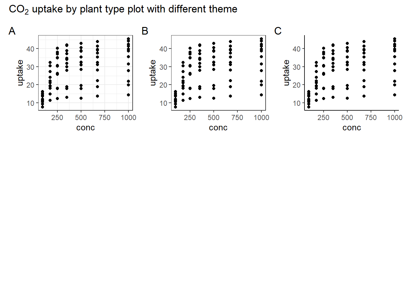
library(ggplot2)
bw <- ggplot(CO2) + geom_point(aes(conc, uptake)) + theme_bw()
test <- ggplot(CO2) + geom_point(aes(conc, uptake)) + theme_test()
classic <- ggplot(CO2) + geom_point(aes(conc, uptake)) + theme_classic()
library(patchwork)
bw + test + classic +
  plot_layout(ncol = 3, widths = c(1, 1, 1), heights = c(1, 1, 1)) +
  plot_annotation(
    title = expression(CO[2] * " uptake by plant type plot with different theme"),
    tag_levels = "A"
  )
5.2 Math formulas with R
head(CO2)Grouped Data: uptake ~ conc | Plant
Plant Type Treatment conc uptake
1 Qn1 Quebec nonchilled 95 16.0
2 Qn1 Quebec nonchilled 175 30.4
3 Qn1 Quebec nonchilled 250 34.8
4 Qn1 Quebec nonchilled 350 37.2
5 Qn1 Quebec nonchilled 500 35.3
6 Qn1 Quebec nonchilled 675 39.2# fundamental expression
plot(CO2$conc, CO2$uptake, pch = 16, las = 1,
xlab = 'CO2 concentration', ylab = 'CO2 uptake')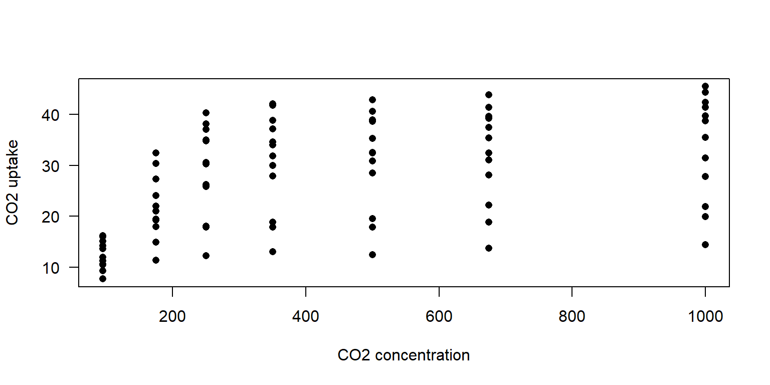
# Advanced expression (Use `?plotmath` to check more details of mathematical annotation in R)
plot(CO2$conc, CO2$uptake, pch = 16, las = 1,
     xlab = expression('CO'[2] * ' concentration (mL/L)'),
     ylab = expression('CO'[2] * ' uptake (' *mu * 'mol m'^-2 * 's'^-1 * ')'))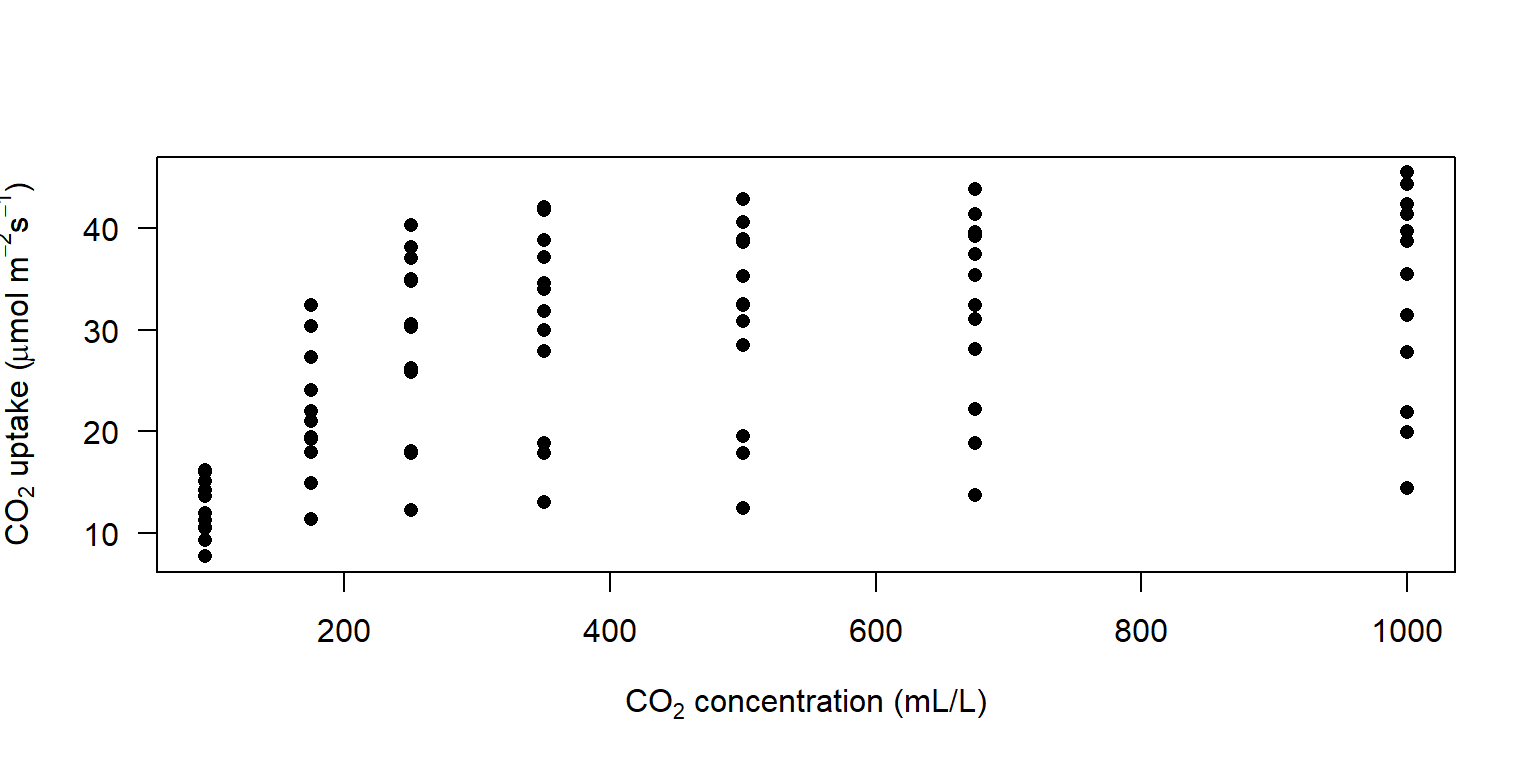
# LaTeX expression
library(latex2exp)
plot(CO2$conc, CO2$uptake, pch = 16, las = 1,
     xlab = TeX('CO$_2$ concentration (mL/L)'),
     ylab = TeX('CO$_2$ uptake ($\\mu$mol m$^{-2}$ s$^{-1}$)'))
text(850, 30, expression(prod(plain(P)(X == x), x)))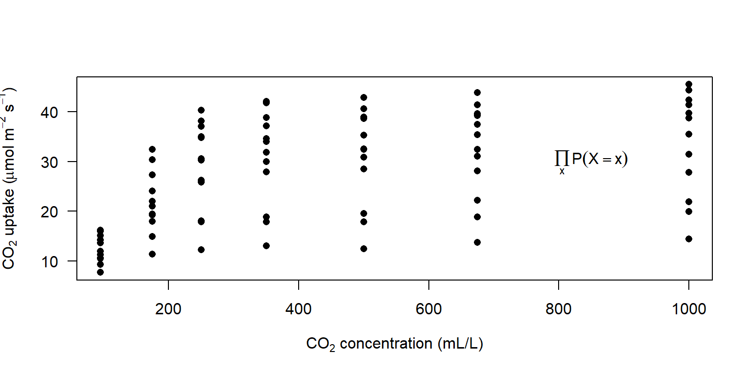
5.3 Size and layout
- ggplot2: patchwork package is used to range the size and layout of multiply plots
library(patchwork)
p1 <- ggplot(airquality) + geom_boxplot(aes(as.factor(Month), Ozone))
p2 <- ggplot(airquality) + geom_point(aes(Solar.R, Ozone))
p3 <- ggplot(airquality) + geom_histogram(aes(Ozone))
p1 + p2 + p3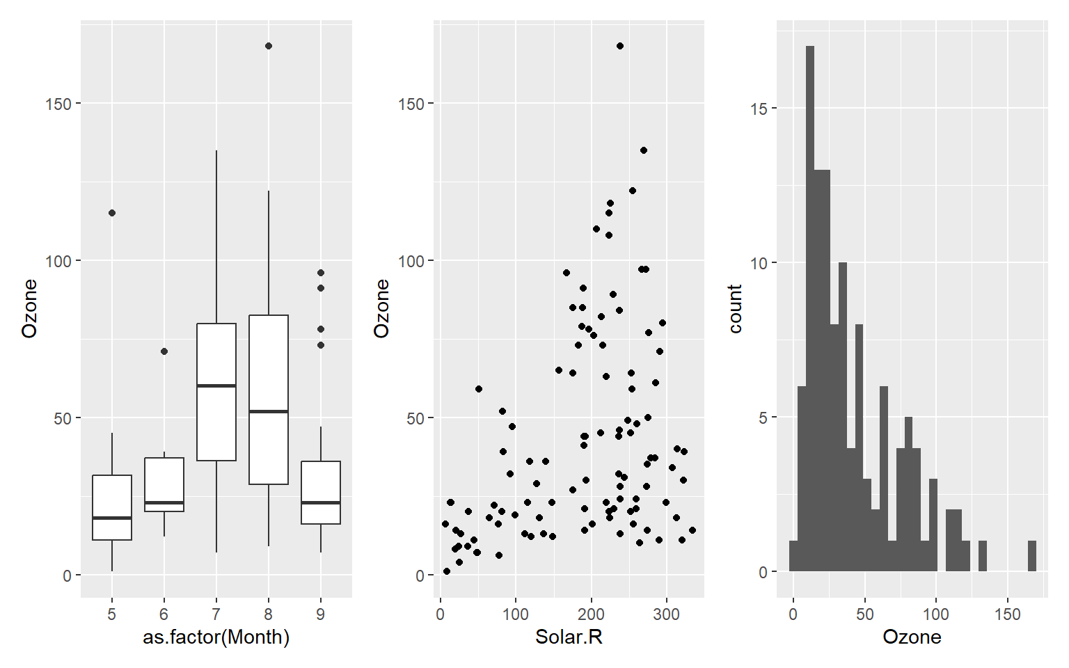
p1 + p2 / p3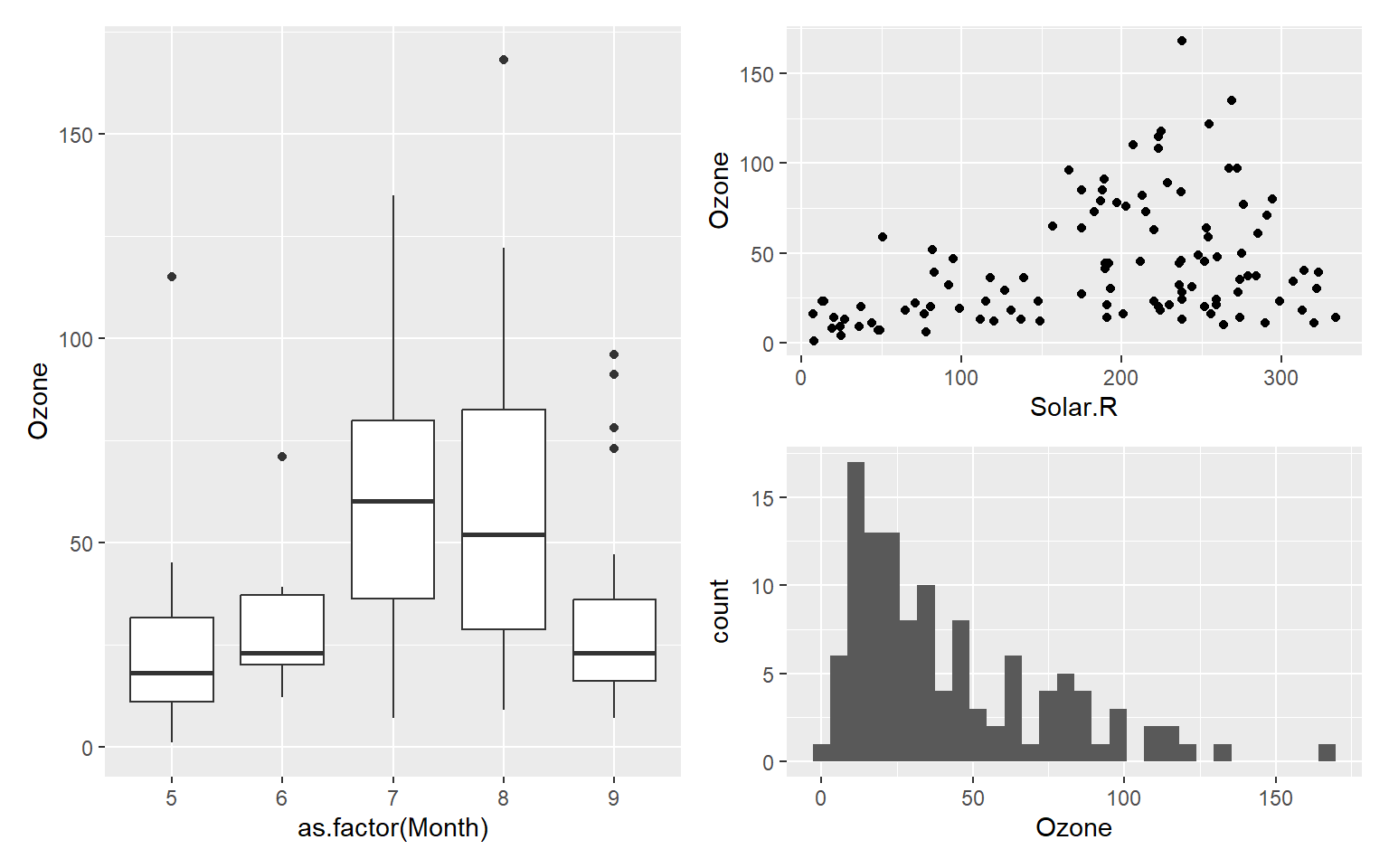
(p1 + p2) / p3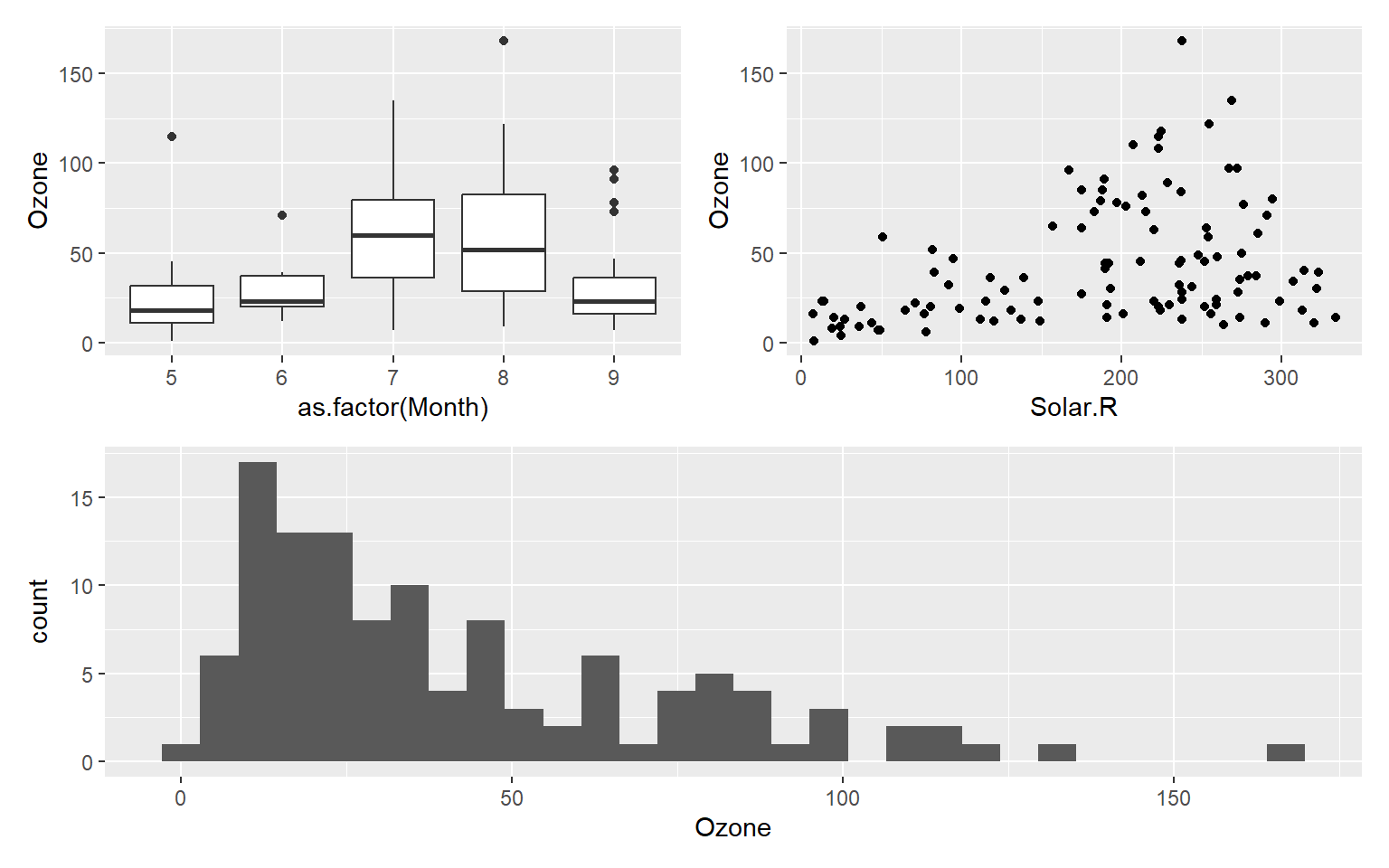
(p1 + p2) / p3 + plot_annotation(tag_levels = 'A') +
  plot_layout(ncol = 2, widths = c(1, 1), heights = c(1, 1))  # plot_layout() function is used to define the grid layout of the composite graph.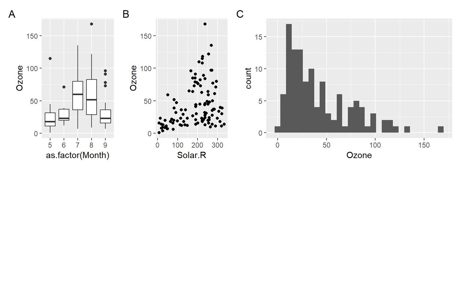
- Built-in par() function
par(mfrow = c(2, 3))  # Set the layout by using vector c(x, y)
plot(airquality$Solar.R, airquality$Ozone)
hist(airquality$Solar.R)
barplot(airquality$Month)
plot(airquality$Solar.R, airquality$Ozone)
hist(airquality$Solar.R)
barplot(airquality$Month)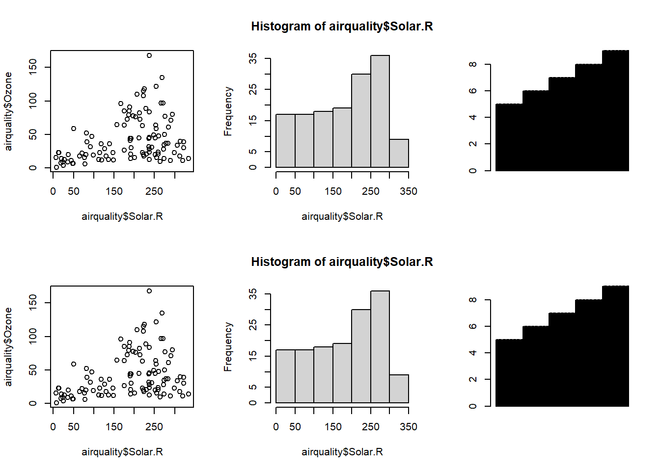
- Built-in layout() function
# Use a matrix to store the information about layout
mymat <- matrix(1:6, nrow = 2)
layout(mymat)
plot(airquality$Solar.R, airquality$Ozone)
hist(airquality$Solar.R)
barplot(airquality$Month)
plot(airquality$Solar.R, airquality$Ozone)
hist(airquality$Solar.R)
barplot(airquality$Month)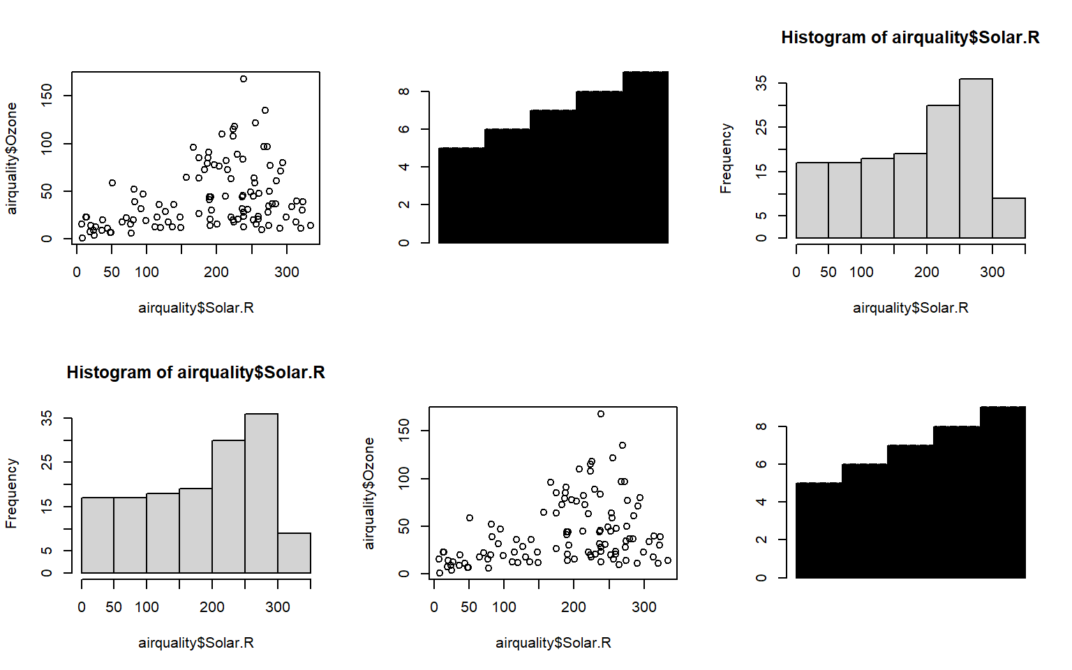
# Also, customize the exact layout by using some parameters like 'widths=' and 'heights=' by filling vector
mymat <- matrix(c(1, 1:5), nrow = 2)
mymat  # Check the matrix which was used to layout plots
[,1] [,2] [,3]
[1,] 1 2 4
[2,] 1 3 5layout(mymat, widths = c(1, 1, 2), heights = c(1, 2))
plot(airquality$Solar.R, airquality$Ozone)
hist(airquality$Solar.R)
barplot(airquality$Month)
plot(airquality$Solar.R, airquality$Ozone)
hist(airquality$Solar.R)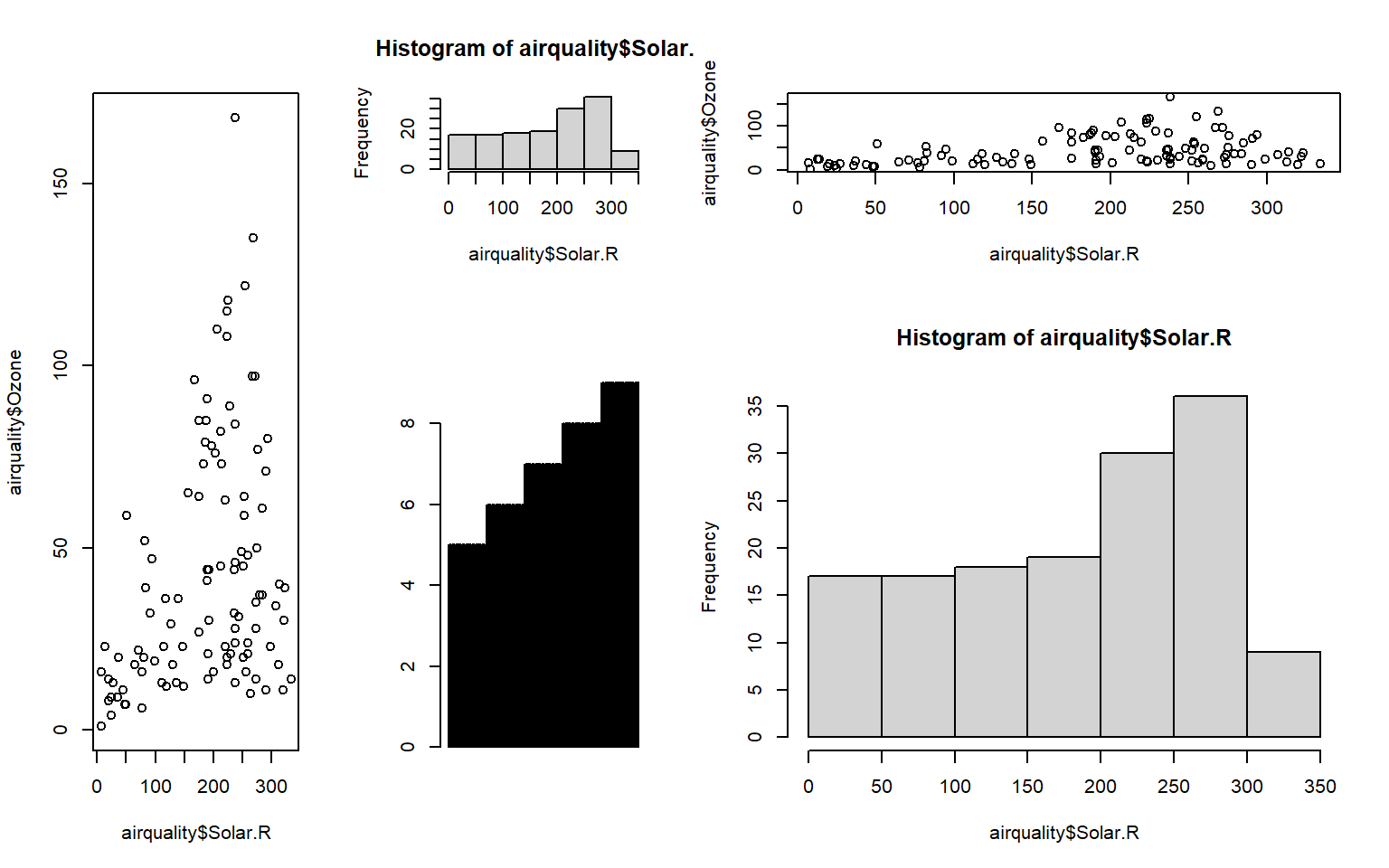
# This is an example from quiz1. Also, please check the exercises to view more difficult questions
mymat <- matrix(c(1, 2, 3, 0), nrow = 2)
mymat  # Check the matrix which was used to layout plots
[,1] [,2]
[1,] 1 3
[2,] 2 0layout(mymat, widths = c(4, 1), heights = c(2, 1)) # Set the ratio between widths and heights
plot(iris$Sepal.Length, iris$Sepal.Width, pch=20, xlab='Sepal Length (cm)', ylab='Sepal Width (cm)', las=1)
boxplot(iris$Sepal.Length, pch=20, las=1, horizontal=T)
boxplot(iris$Sepal.Width, pch=20, las=2)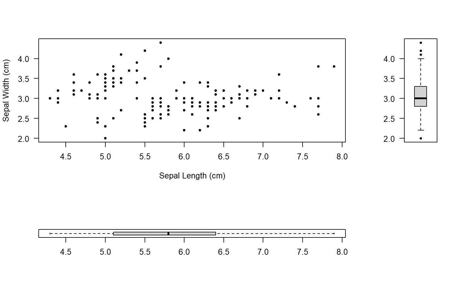
6 R Tidyverse
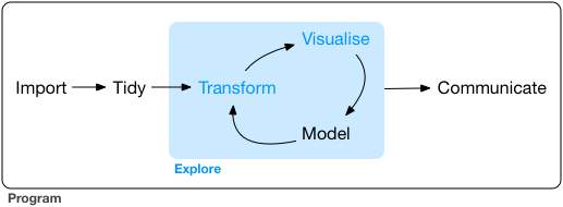
6.1 Workflow
6.2 Fundamental operations
# Load the package
library(tidyverse)
# Check the members of them
tidyverse_packages()
[1] "broom" "conflicted" "cli" "dbplyr"
[5] "dplyr" "dtplyr" "forcats" "ggplot2"
[9] "googledrive" "googlesheets4" "haven" "hms"
[13] "httr" "jsonlite" "lubridate" "magrittr"
[17] "modelr" "pillar" "purrr" "ragg"
[21] "readr" "readxl" "reprex" "rlang"
[25] "rstudioapi" "rvest" "stringr" "tibble"
[29] "tidyr" "xml2" "tidyverse" Core members and their function:
ggplot2: Creating graphicsdplyr: Data manipulationtidyr: Get to tidy datareadr: Read rectangular datapurrr: Functional programmingtibble: Re-imagining of the data framestringr: Working with stringsforcats: Working with factors
6.3 Pipe operator
The pipe operator can be written as %>% or |>
x <- c(0.109, 0.359, 0.63, 0.996, 0.515, 0.142, 0.017, 0.829, 0.907)
# Method 1:
y1 <- log(x)
y2 <- diff(y1)
y3 <- exp(y2)
z <- round(y3)
# Method 2
z <- round(exp(diff(log(x))))
# Pipe method
z <- x %>% log() %>% diff() %>% exp() %>% round()
6.4 Mutiply work by using tidyverse pipe
6.4.1 Graph work
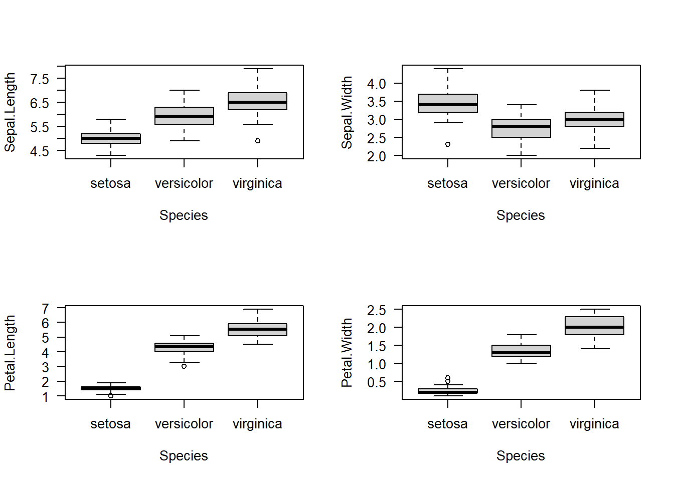
# By using R built-in par() function and a loop
par(mfrow = c(2, 2))
for (i in 1:4) {
  boxplot(iris[, i] ~ iris$Species, las = 1, xlab = 'Species', ylab = names(iris)[i])
}
# By using pivot_longer() function and tidyverse pipe
iris |> pivot_longer(-Species) |> ggplot() + geom_boxplot(aes(Species, value)) + facet_wrap(name ~.)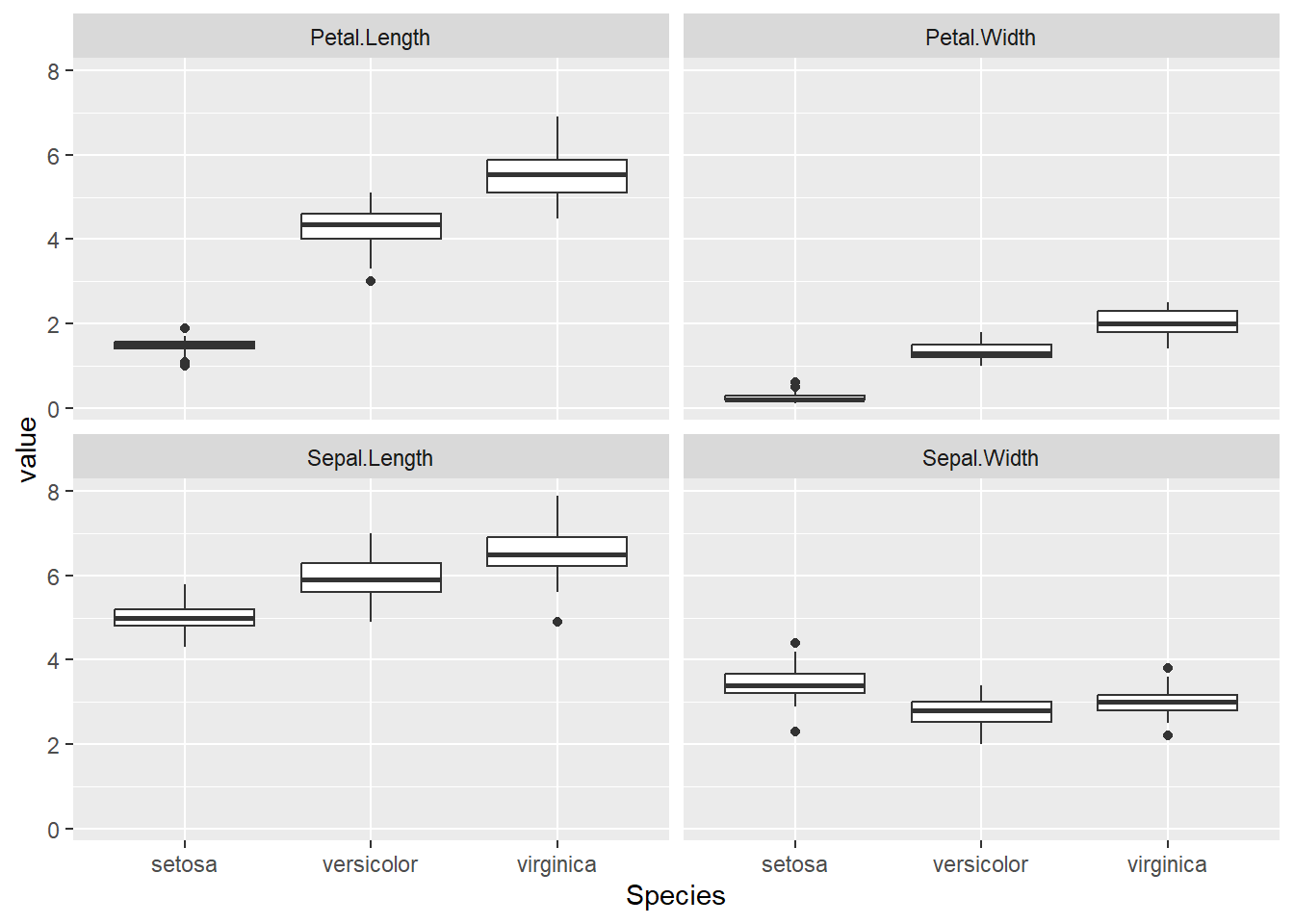
6.4.2 Statistic work
# base R
dtf1_mean <- data.frame(Species = unique(iris$Species), Mean_Sepal_Length = tapply(iris$Sepal.Length, iris$Species, mean, na.rm = TRUE))
dtf1_sd <- data.frame(Species = unique(iris$Species), SD_Sepal_Length = tapply(iris$Sepal.Length, iris$Species, sd, na.rm = TRUE))
dtf1_median <- data.frame(Species = unique(iris$Species), Median_Sepal_Length = tapply(iris$Sepal.Length, iris$Species, median, na.rm = TRUE))
names(dtf1_mean) <- c("Species", "Mean_Sepal_Length")
names(dtf1_sd) <- c("Species", "SD_Sepal_Length")
names(dtf1_median) <- c("Species", "Median_Sepal_Length")
cbind(dtf1_mean, dtf1_sd, dtf1_median)  # Show them in one table
Species Mean_Sepal_Length Species SD_Sepal_Length Species
setosa setosa 5.006 setosa 0.3524897 setosa
versicolor versicolor 5.936 versicolor 0.5161711 versicolor
virginica virginica 6.588 virginica 0.6358796 virginica
Median_Sepal_Length
setosa 5.0
versicolor 5.9
virginica 6.5# use a loop
dtf <- data.frame(rep(NA, 3))
for (i in 1:4) {
dtf1_mean <- data.frame(tapply(iris[, i], iris$Species, mean, na.rm = TRUE))
dtf1_sd <- data.frame(tapply(iris[, i], iris$Species, sd, na.rm = TRUE))
dtf1_median <- data.frame(tapply(iris[, i], iris$Species, median, na.rm = TRUE))
dtf1 <- cbind(dtf1_mean, dtf1_sd, dtf1_median)
names(dtf1) <- paste0(names(iris)[i], '.', c('mean', 'sd', 'median'))
dtf <- cbind(dtf, dtf1)
}
dtf rep.NA..3. Sepal.Length.mean Sepal.Length.sd Sepal.Length.median
setosa NA 5.006 0.3524897 5.0
versicolor NA 5.936 0.5161711 5.9
virginica NA 6.588 0.6358796 6.5
Sepal.Width.mean Sepal.Width.sd Sepal.Width.median Petal.Length.mean
setosa 3.428 0.3790644 3.4 1.462
versicolor 2.770 0.3137983 2.8 4.260
virginica 2.974 0.3224966 3.0 5.552
Petal.Length.sd Petal.Length.median Petal.Width.mean Petal.Width.sd
setosa 0.1736640 1.50 0.246 0.1053856
versicolor 0.4699110 4.35 1.326 0.1977527
virginica 0.5518947 5.55 2.026 0.2746501
Petal.Width.median
setosa 0.2
versicolor 1.3
virginica 2.0# tidyverse
dtf <- iris |>
pivot_longer(-Species) |>
group_by(Species, name) |>
summarise(mean = mean(value, na.rm = TRUE),
sd = sd(value, na.rm = TRUE),
median = median(value, na.rm = TRUE),
.groups = "drop")
dtf# A tibble: 12 × 5
Species name mean sd median
<fct> <chr> <dbl> <dbl> <dbl>
1 setosa Petal.Length 1.46 0.174 1.5
2 setosa Petal.Width 0.246 0.105 0.2
3 setosa Sepal.Length 5.01 0.352 5
4 setosa Sepal.Width 3.43 0.379 3.4
5 versicolor Petal.Length 4.26 0.470 4.35
6 versicolor Petal.Width 1.33 0.198 1.3
7 versicolor Sepal.Length 5.94 0.516 5.9
8 versicolor Sepal.Width 2.77 0.314 2.8
9 virginica Petal.Length 5.55 0.552 5.55
10 virginica Petal.Width 2.03 0.275 2
11 virginica Sepal.Length 6.59 0.636 6.5
12 virginica Sepal.Width 2.97 0.322 3 6.5 Tidy the dataset
# Original dataset of table1
table1
# A tibble: 6 × 4
country year cases population
<chr> <dbl> <dbl> <dbl>
1 Afghanistan 1999 745 19987071
2 Afghanistan 2000 2666 20595360
3 Brazil 1999 37737 172006362
4 Brazil 2000 80488 174504898
5 China 1999 212258 1272915272
6 China 2000 213766 1280428583# Compute rate per 10,000
table1 %>% mutate(rate = cases / population * 10000)# A tibble: 6 × 5
country year cases population rate
<chr> <dbl> <dbl> <dbl> <dbl>
1 Afghanistan 1999 745 19987071 0.373
2 Afghanistan 2000 2666 20595360 1.29
3 Brazil 1999 37737 172006362 2.19
4 Brazil 2000 80488 174504898 4.61
5 China 1999 212258 1272915272 1.67
6 China 2000 213766 1280428583 1.67 # Compute cases per year
table1 %>% count(year, wt = cases)# A tibble: 2 × 2
year n
<dbl> <dbl>
1 1999 250740
2 2000 2969206.6 Conversions the dataframe type
# Original dataset of table2
table2
# A tibble: 12 × 4
country year type count
<chr> <dbl> <chr> <dbl>
1 Afghanistan 1999 cases 745
2 Afghanistan 1999 population 19987071
3 Afghanistan 2000 cases 2666
4 Afghanistan 2000 population 20595360
5 Brazil 1999 cases 37737
6 Brazil 1999 population 172006362
7 Brazil 2000 cases 80488
8 Brazil 2000 population 174504898
9 China 1999 cases 212258
10 China 1999 population 1272915272
11 China 2000 cases 213766
12 China 2000 population 1280428583# Divided the type into cases and population
table2 %>% pivot_wider(names_from = type, values_from = count)# A tibble: 6 × 4
country year cases population
<chr> <dbl> <dbl> <dbl>
1 Afghanistan 1999 745 19987071
2 Afghanistan 2000 2666 20595360
3 Brazil 1999 37737 172006362
4 Brazil 2000 80488 174504898
5 China 1999 212258 1272915272
6 China 2000 213766 1280428583# Original dataset of table3
table3# A tibble: 6 × 3
country year rate
<chr> <dbl> <chr>
1 Afghanistan 1999 745/19987071
2 Afghanistan 2000 2666/20595360
3 Brazil 1999 37737/172006362
4 Brazil 2000 80488/174504898
5 China 1999 212258/1272915272
6 China 2000 213766/1280428583# Separate the rate into cases and population
table3 %>% separate(col = rate, into = c("cases", "population"), sep = "/")# A tibble: 6 × 4
country year cases population
<chr> <dbl> <chr> <chr>
1 Afghanistan 1999 745 19987071
2 Afghanistan 2000 2666 20595360
3 Brazil 1999 37737 172006362
4 Brazil 2000 80488 174504898
5 China 1999 212258 1272915272
6 China 2000 213766 1280428583# Original dataset of table4a and table4b
cbind(table4a, table4b) country 1999 2000 country 1999 2000
1 Afghanistan 745 2666 Afghanistan 19987071 20595360
2 Brazil 37737 80488 Brazil 172006362 174504898
3 China 212258 213766 China 1272915272 1280428583# Put table4a and table4b together to form a new table with both of their dataset
tidy4a_changed <- table4a %>% pivot_longer(c(`1999`, `2000`), names_to = "year", values_to = "cases")
tidy4b_changed <- table4b %>% pivot_longer(c(`1999`, `2000`), names_to = "year", values_to = "population")
left_join(tidy4a_changed, tidy4b_changed) ## Kind of like MySQL# A tibble: 6 × 4
country year cases population
<chr> <chr> <dbl> <dbl>
1 Afghanistan 1999 745 19987071
2 Afghanistan 2000 2666 20595360
3 Brazil 1999 37737 172006362
4 Brazil 2000 80488 174504898
5 China 1999 212258 1272915272
6 China 2000 213766 12804285836.7 Find missing observations
library(openair)
library(tidyverse)
# create a function to count missing observations
sum_of_na <- function(x){
  sum(is.na(x))
}
mydata %>% summarise(
  across(everything(), sum_of_na)
)
# A tibble: 1 × 10
date ws wd nox no2 o3 pm10 so2 co pm25
<int> <int> <int> <int> <int> <int> <int> <int> <int> <int>
1 0 632 219 2423 2438 2589 2162 10450 1936 87757 ANOVA (Post-hoc tests)
7.1 Post-hoc tests
Background informations: A biologist studies the weight gain of male lab rats on diets over a 4-week period. Three different diets are applied.
# Statistic anlysis
(dtf <- data.frame(diet1 = c(90, 95, 100),
                   diet2 = c(120, 125, 130),
                   diet3 = c(125, 130, 135)))
diet1 diet2 diet3
1 90 120 125
2 95 125 130
3 100 130 135dtf2 <- stack(dtf)
names(dtf2) <- c("wg", "diet")
wg_aov <- aov(wg ~ diet, data = dtf2)
summary(wg_aov) Df Sum Sq Mean Sq F value Pr(>F)
diet 2 2150 1075 43 0.000277 ***
Residuals 6 150 25
---
Signif. codes: 0 '***' 0.001 '**' 0.01 '*' 0.05 '.' 0.1 ' ' 1# Visualization
library(ggplot2)
ggplot(dtf2) + geom_boxplot(aes(wg, diet))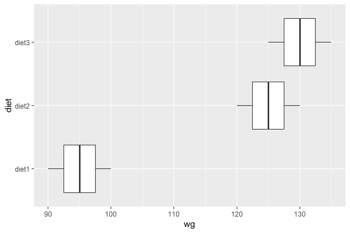
7.2 Fisher’s Least Significant Difference (LSD) Test
7.2.1 Concept
Pair-wise comparisons of all the groups based on the \(t\)-test: \[L S D=t_{\alpha / 2} \sqrt{S_{p}^{2}\left(\frac{1}{n_1}+\frac{1}{n_2}+\cdots\right)}\] \[S_{p}^{2}=\frac{\left(n_{1}-1\right) S_{1}^{2}+\left(n_{2}-1\right) S_{2}^{2}+\left(n_{3}-1\right) S_{3}^{2}+\cdots}{\left(n_{1}-1\right)+\left(n_{2}-1\right)+\left(n_{3}-1\right)+\cdots}\]
- \(S_{p}^{2}:\): pooled standard deviation (some use Mean Standard Error)
- \(t_{\alpha / 2}: \mathrm{t}\): \(t\) critical value at \(\alpha=0.025\)
- Degree of freedom: \(N - k\)
- \(N\): total observations
- \(k\): number of factors
- If \(\left|\bar{x}_{1}-\bar{x}_{2}\right|>L S D\), then the difference of \(x_1\) group and \(x_2\) group is significant at \(\alpha\).
- In multiple comparisons (\(k\) factors), the number of comparison needed is: \(\frac{k(k-1)}{2}\)
7.2.2 Example
(Rats on diets in the previous section)
- Step by step
# Calculate LSD
n <- nrow(dtf2)
k <- nlevels(dtf2$diet)
dfree <- n - k
t_critical <- qt(0.05/2, df = dfree, lower.tail = FALSE)
sp2 <- sum((3 - 1) * apply(dtf, 2, sd) ^ 2)/ dfree
LSD <- t_critical * sqrt(sp2 * (1/3 + 1/3 + 1/3))
# Calculate |mean_x1-mean_x2|
dtf_groupmean <- colMeans(dtf)
paired_groupmean <- combn(dtf_groupmean, 2)
paired_groupmean[2, ] - paired_groupmean[1, ]
[1] 30 35 5LSD[1] 12.23456- Step by step by using loop
library(dplyr)
dtf_sm <- dtf2 |>
  group_by(diet) |>
  summarise(n = length(wg), sd = sd(wg), mean = mean(wg))
sp2 <- sum((dtf_sm$n - 1) * dtf_sm$sd ^ 2 )/ dfree
LSD <- t_critical * sqrt(sp2 * sum(1 / dtf_sm$n))
paired_groupmean <- combn(dtf_sm$mean, 2)
paired_groupmean[2, ] - paired_groupmean[1, ]
[1] 30 35 5- One step
library(agricolae)
# Statistic analysis
LSD.test(wg_aov, "diet", p.adj = "bonferroni") |> print()
$statistics
MSerror Df Mean CV t.value MSD
25 6 116.6667 4.285714 3.287455 13.42098
$parameters
test p.ajusted name.t ntr alpha
Fisher-LSD bonferroni diet 3 0.05
$means
wg std r LCL UCL Min Max Q25 Q50 Q75
diet1 95 5 3 87.93637 102.0636 90 100 92.5 95 97.5
diet2 125 5 3 117.93637 132.0636 120 130 122.5 125 127.5
diet3 130 5 3 122.93637 137.0636 125 135 127.5 130 132.5
$comparison
NULL
$groups
wg groups
diet3 130 a
diet2 125 a
diet1 95 b
attr(,"class")
[1] "group"The meaning of each parameter in this table
- $statistics:包含ANOVA分析的统计量(statistics)的列表。
- MSerror:平均方差误差(mean square error),也称为残差方差,表示模型误差的平均程度。
- Df:自由度(degrees of freedom)。
- Mean:均值(mean)。
- CV:变异系数(coefficient of variation),变异系数越大,说明数据的离散程度越大。
- t.value:t值(t-value),表示组间均值之间的显著性差异程度。
- MSD:最小显著差异(minimum significant difference),表示在显著性水平下两个组之间的最小显著差异值。
- $parameters:包含对比分析的参数(parameters)的列表。
- test:所使用的多重比较方法(multiple comparison method),此处为Fisher-LSD法。
- p.ajusted:经过校正后的显著性水平(adjusted significance level),此处为Bonferroni法。 -name.t:所进行对比分析的因素名称(name of tested factor),此处为diet。
- ntr:因素水平数(number of treatments),此处为3。
- alpha:显著性水平(significance level),此处为0.05。
- $means:包含各组均值和统计信息(means and statistics)的列表。
- wg:组均值(group mean)。
- std:标准差(standard deviation)。
- r:重复次数(replications)。
- LCL:下限置信区间(lower confidence limit)。
- UCL:上限置信区间(upper confidence limit)。
- Min:最小值(minimum value)。
- Max:最大值(maximum value)。
- Q25:25%分位数(25th percentile)。
- Q50:50%分位数(50th percentile),也称为中位数。
- Q75:75%分位数(75th percentile)。
- $comparison:对比分析结果(comparison),此处为空。
- $groups:分组结果(groups)。
- wg:组均值(group mean)。
- groups:分组结果(groups),使用字母表示不同组别,相同字母表示在统计上没有显著差异。
- attr(,“class”):结果的类别(class),此处为”group”。
# Visualization
LSD.test(wg_aov, "diet", p.adj = "bonferroni") |> plot()
box()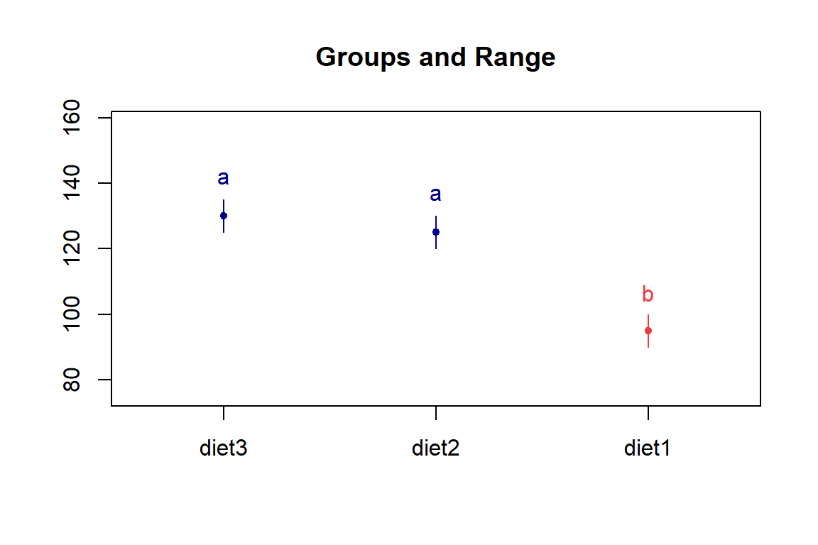
Conclusion: At \(\alpha = 0.05\), Diet 2 and Diet 3 are significantly different from Diet 1 in the mean weight gain, while Diet 2 is not significantly different from Diet 3.
7.3 Bonferroni t-test
7.3.1 Concept
A multiple-comparison post-hoc test, which sets the significance cut off at \(\alpha/m\) for each comparison, where \(m\) represents the number of comparisons we apply.
Overall chance of making a Type I error:
m <- 1:100
siglevel <- 0.05
Type_I <- 1 - (1 - (siglevel / m)) ^ m
Type_I
[1] 0.05000000 0.04937500 0.04917130 0.04907029 0.04900995 0.04896984
[7] 0.04894124 0.04891982 0.04890317 0.04888987 0.04887899 0.04886993
[13] 0.04886227 0.04885571 0.04885002 0.04884504 0.04884065 0.04883675
[19] 0.04883326 0.04883012 0.04882728 0.04882470 0.04882235 0.04882019
[25] 0.04881820 0.04881637 0.04881467 0.04881309 0.04881162 0.04881025
[31] 0.04880897 0.04880777 0.04880664 0.04880558 0.04880458 0.04880363
[37] 0.04880274 0.04880189 0.04880109 0.04880033 0.04879960 0.04879891
[43] 0.04879825 0.04879762 0.04879702 0.04879644 0.04879589 0.04879536
[49] 0.04879486 0.04879437 0.04879390 0.04879346 0.04879302 0.04879261
[55] 0.04879221 0.04879182 0.04879145 0.04879109 0.04879074 0.04879040
[61] 0.04879008 0.04878976 0.04878946 0.04878916 0.04878888 0.04878860
[67] 0.04878833 0.04878807 0.04878782 0.04878757 0.04878733 0.04878710
[73] 0.04878687 0.04878665 0.04878644 0.04878623 0.04878602 0.04878583
[79] 0.04878563 0.04878544 0.04878526 0.04878508 0.04878491 0.04878474
[85] 0.04878457 0.04878441 0.04878425 0.04878409 0.04878394 0.04878379
[91] 0.04878365 0.04878350 0.04878337 0.04878323 0.04878310 0.04878297
[97] 0.04878284 0.04878271 0.04878259 0.048782477.3.2 Example
(Rats on diets in the previous section)
- Step by step
m <- choose(nlevels(dtf2$diet), 2)  # 1:2 or 1:3 or 2:3
alpha_cor <- 0.05 / m
# Pairwise comparison between diet1 and diet2
t.test(wg ~ diet, dtf2, subset = diet %in% c("diet1", "diet2"), conf.level = 1 - alpha_cor)
    Welch Two Sample t-test

data:  wg by diet
t = -7.3485, df = 4, p-value = 0.001826
alternative hypothesis: true difference in means between group diet1 and group diet2 is not equal to 0
98.33333 percent confidence interval:
 -46.16984 -13.83016
sample estimates:
mean in group diet1 mean in group diet2
                 95                 125
# Pairwise comparison between diet1 and diet3
t.test(wg ~ diet, dtf2, subset = diet %in% c("diet1", "diet3"), conf.level = 1 - alpha_cor)
    Welch Two Sample t-test

data:  wg by diet
t = -8.5732, df = 4, p-value = 0.001017
alternative hypothesis: true difference in means between group diet1 and group diet3 is not equal to 0
98.33333 percent confidence interval:
 -51.16984 -18.83016
sample estimates:
mean in group diet1 mean in group diet3
                 95                 130
# Pairwise comparison between diet2 and diet3
t.test(wg ~ diet, dtf2, subset = diet %in% c("diet2", "diet3"), conf.level = 1 - alpha_cor)
    Welch Two Sample t-test

data:  wg by diet
t = -1.2247, df = 4, p-value = 0.2879
alternative hypothesis: true difference in means between group diet2 and group diet3 is not equal to 0
98.33333 percent confidence interval:
 -21.16984  11.16984
sample estimates:
mean in group diet2 mean in group diet3
125 130 - One step
(diet_pt <- pairwise.t.test(dtf2$wg, dtf2$diet, pool.sd = FALSE,var.equal = TRUE, p.adj = "none"))
    Pairwise comparisons using t tests with non-pooled SD

data:  dtf2$wg and dtf2$diet

      diet1  diet2
diet2 0.0018 -
diet3 0.0010 0.2879

P value adjustment method: none diet_pt$p.value < 0.05 diet1 diet2
diet2 TRUE NA
diet3 TRUE FALSEConclusion: At \(\alpha = 0.05\), Diet 2 and Diet 3 are significantly different from Diet 1 in the mean weight gain, while Diet 2 is not significantly different from Diet 3.
8 MANOVA

8.1 Definition
Univariate Analysis of Variance (ANOVA):
- one dependent variable (continuous) ~ one or multiple independent variables (categorical).
Multivariate Analysis of Variance (MANOVA)
- multiple dependent variables (continuous) ~ one or multiple independent variables (categorical).
Comparing multivariate sample means. It uses the covariance between outcome variables in testing the statistical significance of the mean differences when there are multiple dependent variables.
Merit of MANOVA:
- Reduce the Type I error
- It allows for the analysis of multiple dependent variables simultaneously
- It provides information about the strength and direction of relationships
8.2 Workflow
Example: Influence of teaching methods on student satisfaction scores and exam scores.
dtf <- read.csv('data/teaching_methods.csv')
head(dtf, 3)
Method Test Satisfaction
1 1 3.000 3.001
2 1 2.990 2.994
3 1 3.041 3.032# ANOVA between Test and Method
summary(aov(Test ~ Method, data = dtf)) Df Sum Sq Mean Sq F value Pr(>F)
Method 1 0.000578 0.0005780 2.426 0.126
Residuals 46 0.010958 0.0002382 # ANOVA between Satisfaction and Method
summary(aov(Satisfaction ~ Method, data = dtf)) Df Sum Sq Mean Sq F value Pr(>F)
Method 1 0.000032 0.0000320 0.135 0.715
Residuals 46 0.010944 0.0002379 # Visualization with Scatter plot
library(ggplot2)
library(tidyr)
dtf |> pivot_longer(-Method) |>
ggplot() +
geom_dotplot(aes(x = Method, y = value, group = Method), binaxis = "y", stackdir = "center") +
facet_wrap(name~.)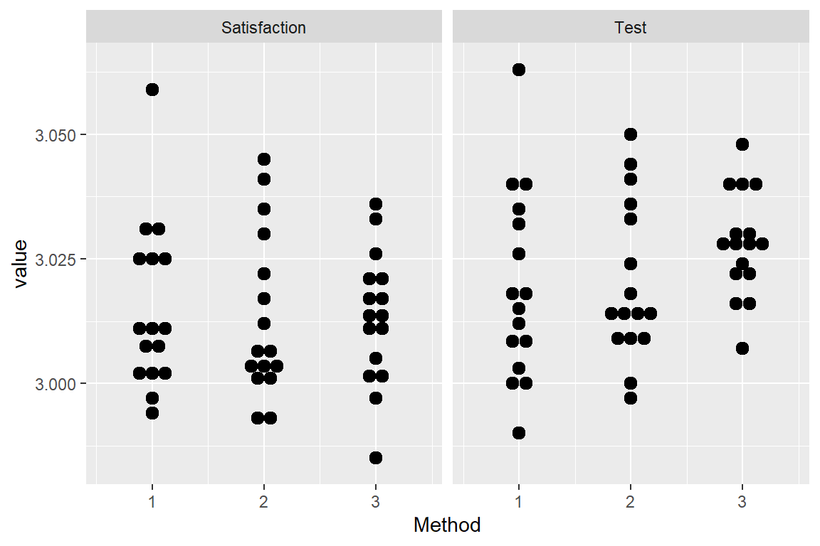
# Visualization with Box plot
par(mfrow = c(1, 3))
boxplot(Test ~ Method, data = dtf)
boxplot(Satisfaction ~ Method, data = dtf)
plot(dtf$Satisfaction, dtf$Test, col = dtf$Method, pch = 16, xlab = 'Satisfaction', ylab = 'Test')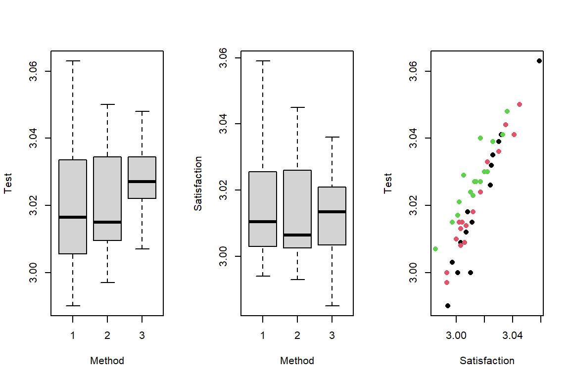
# MANOVA method: use manova() function with multiple response variables ~ one or multiple factor
# column bind way
tm_manova <- manova(cbind(dtf$Test, dtf$Satisfaction) ~ dtf$Method)
# matrix way
tm_manova <- manova(as.matrix(dtf[, c('Test', 'Satisfaction')]) ~ dtf$Method)
summary(tm_manova)
Df Pillai approx F num Df den Df Pr(>F)
dtf$Method 1 0.45766 18.987 2 45 1.05e-06 ***
Residuals 46
---
Signif. codes: 0 '***' 0.001 '**' 0.01 '*' 0.05 '.' 0.1 ' ' 18.3 One-way MANOVA

Example: The iris dataset. Do the species have influence on the sepal size?
# Visualization
library(ggplot2)
library(tidyr)
iris[, c('Species', 'Sepal.Length', 'Sepal.Width')] |>
  pivot_longer(cols = c(Sepal.Length, Sepal.Width)) |>
  ggplot() +
  geom_boxplot(aes(Species, value, fill = name)) +
  labs(y = 'Size (cm)', fill = '')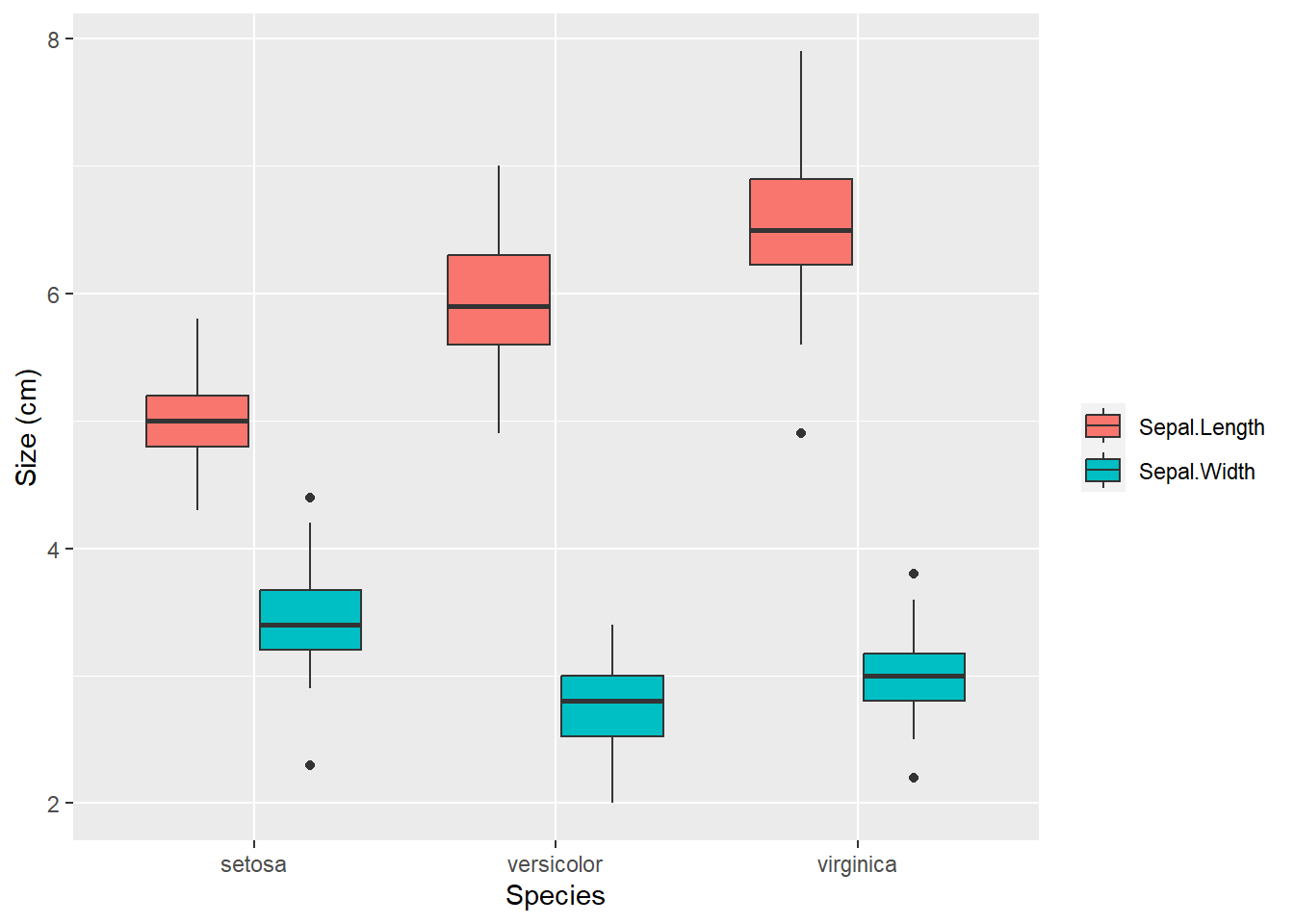
library(gplots)
par(mfrow = c(1, 2))
plotmeans(iris$Sepal.Length ~ iris$Species, xlab = "Species", ylab = "Sepal length")
plotmeans(iris$Sepal.Width ~ iris$Species, xlab = "Species", ylab = "Sepal width")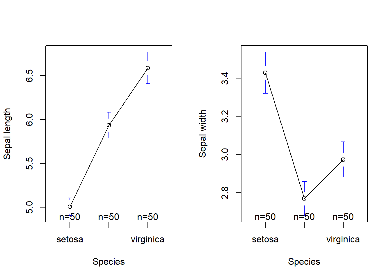
Hypothesis: multivariate normality test
- \(H_0\): The population means of the sepal length and the sepal width are not different across the species.
# Summary MANOVA result with different test method
SepalSize <- cbind(iris$Sepal.Length, iris$Sepal.Width)
iris_manova <- manova(SepalSize ~ iris$Species)summary(iris_manova, test = 'Pillai') # default Df Pillai approx F num Df den Df Pr(>F)
iris$Species 2 0.94531 65.878 4 294 < 2.2e-16 ***
Residuals 147
---
Signif. codes: 0 '***' 0.001 '**' 0.01 '*' 0.05 '.' 0.1 ' ' 1summary(iris_manova, test = 'Wilks') Df Wilks approx F num Df den Df Pr(>F)
iris$Species 2 0.16654 105.88 4 292 < 2.2e-16 ***
Residuals 147
---
Signif. codes: 0 '***' 0.001 '**' 0.01 '*' 0.05 '.' 0.1 ' ' 1summary(iris_manova, test = 'Roy') Df Roy approx F num Df den Df Pr(>F)
iris$Species 2 4.1718 306.63 2 147 < 2.2e-16 ***
Residuals 147
---
Signif. codes: 0 '***' 0.001 '**' 0.01 '*' 0.05 '.' 0.1 ' ' 1summary(iris_manova, test = 'Hotelling-Lawley') Df Hotelling-Lawley approx F num Df den Df Pr(>F)
iris$Species 2 4.3328 157.06 4 290 < 2.2e-16 ***
Residuals 147
---
Signif. codes: 0 '***' 0.001 '**' 0.01 '*' 0.05 '.' 0.1 ' ' 1# Univariate ANOVAs for each dependent variable
summary.aov(iris_manova) Response 1 :
Df Sum Sq Mean Sq F value Pr(>F)
iris$Species 2 63.212 31.606 119.26 < 2.2e-16 ***
Residuals 147 38.956 0.265
---
Signif. codes: 0 '***' 0.001 '**' 0.01 '*' 0.05 '.' 0.1 ' ' 1
Response 2 :
Df Sum Sq Mean Sq F value Pr(>F)
iris$Species 2 11.345 5.6725 49.16 < 2.2e-16 ***
Residuals 147 16.962 0.1154
---
Signif. codes: 0 '***' 0.001 '**' 0.01 '*' 0.05 '.' 0.1 ' ' 1Conclusion: The species has a statistically significant effect on the sepal width and sepal length.
8.4 Post-hoc test
Example: after One-way MANOVA gives a significant result, which group(s) is/are different from other(s)?
Hypothesis: Linear Discriminant Analysis (LDA)
# Visualization
library(MASS)
iris_lda <- lda(iris$Species ~ SepalSize, CV = FALSE)
plot_lda <- data.frame(Species = iris$Species, lda = predict(iris_lda)$x)
ggplot(plot_lda) + geom_point(aes(x = lda.LD1, y = lda.LD2, colour = Species))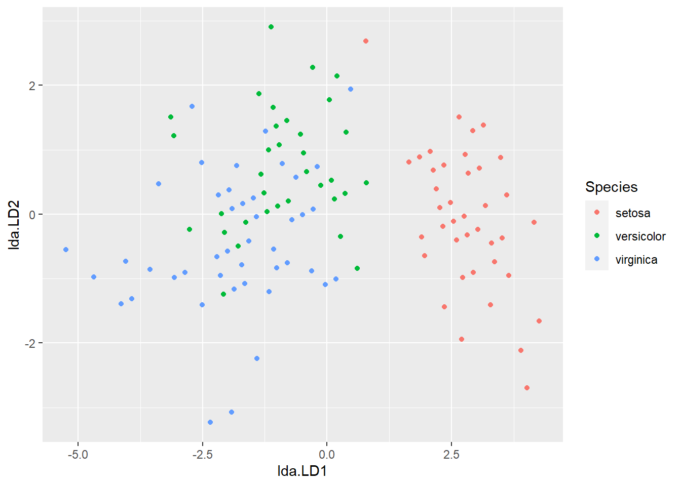
Conclusion: The sepal size of the setosa species is different from other species.
8.5 Multivariate normality
8.5.1 Shapiro-Wilk test
Hypothesis:
\(H_0\): The variable follows a normal distribution
library(rstatix)
iris |>
  group_by(Species) |>
  shapiro_test(Sepal.Length, Sepal.Width)
# A tibble: 6 × 4
Species variable statistic p
<fct> <chr> <dbl> <dbl>
1 setosa Sepal.Length 0.978 0.460
2 setosa Sepal.Width 0.972 0.272
3 versicolor Sepal.Length 0.978 0.465
4 versicolor Sepal.Width 0.974 0.338
5 virginica Sepal.Length 0.971 0.258
6 virginica Sepal.Width 0.967 0.181Tips:
- If the sample size is large (say n > 50), the visual approaches such as QQ-plot and histogram will be better for assessing the normality assumption.
iris[, c('Species', 'Sepal.Length', 'Sepal.Width')] |>
  pivot_longer(cols = c(Sepal.Length, Sepal.Width)) |>
  ggplot() +
  geom_histogram(aes(value)) +
  facet_grid(name ~ Species)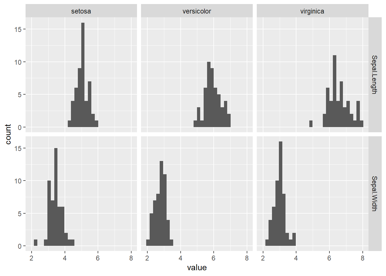
Conclusion: As \(p>0.05\), the sepal length and the width for each species are normally distributed.
8.5.2 Mardia’s skewness and kurtosis test
Hypothesis:
\(H_0\): The variables follow a multivariate normal distribution
library(mvnormalTest)
mardia(iris[, c('Sepal.Length', 'Sepal.Width')])$mv.test
Test Statistic p-value Result
1 Skewness 9.4614 0.0505 YES
2 Kurtosis -0.691 0.4896 YES
3 MV Normality <NA> <NA> YESTip:
- When n > 20 for each combination of the independent and dependent variable, the multivariate normality can be assumed (Multivariate Central Limit Theorem).
Conclusion: As \(p>0.05\), the sepal length and the width follow a multivariate normal distribution.
8.5.3 Homogeneity of the variance-covariance matrix
Main:
Box’s M test: Use a lower \(\alpha\) level such as \(\alpha = 0.001\) to assess the \(p\) value for significance.
Hypothesis:
\(H_0\): The variance-covariance matrices are equal for each combination formed by each group in the independent variable.
library(biotools)
boxM(cbind(iris$Sepal.Length, iris$Sepal.Width), iris$Species)
    Box's M-test for Homogeneity of Covariance Matrices

data:  cbind(iris$Sepal.Length, iris$Sepal.Width)
Chi-Sq (approx.) = 35.655, df = 6, p-value = 3.217e-06
Conclusion: As \(p < 0.001\), the variance-covariance matrices for the sepal length and width are not equal for each combination formed by each species.
8.5.4 Multivariate outliers
- MANOVA is highly sensitive to outliers and may produce Type I or II errors.
- Multivariate outliers can be detected using the Mahalanobis Distance test. The larger the Mahalanobis Distance, the more likely it is an outlier.
library(rstatix)
iris_outlier <- mahalanobis_distance(iris[, c('Sepal.Length', 'Sepal.Width')])
head(iris_outlier, 5)
Sepal.Length Sepal.Width mahal.dist is.outlier
1 5.1 3.5 1.646 FALSE
2 4.9 3.0 1.369 FALSE
3 4.7 3.2 1.934 FALSE
4 4.6 3.1 2.261 FALSE
5 5.0 3.6 2.321 FALSE8.5.5 Linearity
- Or test the regression or the slope (ENV221)
# Visualize the pairwise scatterplot for the dependent variable for each group
ggplot(iris, aes(x = Sepal.Length, y = Sepal.Width)) +
  geom_point() +
  geom_smooth(method = 'lm') +
  facet_wrap(Species ~ .)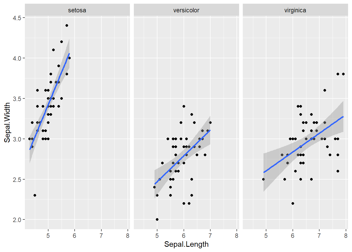
8.5.6 Multicollinearity
Correlation between the dependent variable.
For three or more dependent variables, use a correlation matrix or variance inflation factor (VIF).
# Test the correlation
cor.test(x = iris$Sepal.Length, y = iris$Sepal.Width)
    Pearson's product-moment correlation

data:  iris$Sepal.Length and iris$Sepal.Width
t = -1.4403, df = 148, p-value = 0.1519
alternative hypothesis: true correlation is not equal to 0
95 percent confidence interval:
 -0.27269325  0.04351158
sample estimates:
       cor
-0.1175698
# Visualization
ggplot(iris, aes(Sepal.Length, Sepal.Width)) +
geom_point() +
geom_smooth(method = 'lm')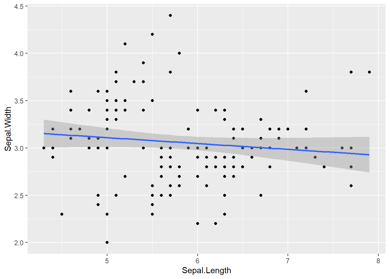
- If \(|r|\) > 0.9, there is multicollinearity.
- If r is too low, perform separate univariate ANOVA for each dependent variable.
8.6 Two-way MANOVA

Example: Plastic. Do the rate of extrusion and the additive have influence on the plastic quality?
# Summary MANOVA result
data('Plastic', package = 'heplots')
Plastic_matrix <- as.matrix(Plastic[, c('tear','gloss','opacity')])
Plastic_manova <- manova(Plastic_matrix ~ Plastic$rate * Plastic$additive)
summary(Plastic_manova)
Df Pillai approx F num Df den Df Pr(>F)
Plastic$rate 1 0.61814 7.5543 3 14 0.003034 **
Plastic$additive 1 0.47697 4.2556 3 14 0.024745 *
Plastic$rate:Plastic$additive 1 0.22289 1.3385 3 14 0.301782
Residuals 16
---
Signif. codes: 0 '***' 0.001 '**' 0.01 '*' 0.05 '.' 0.1 ' ' 1# Univariate ANOVAs for each dependent variable
summary.aov(Plastic_manova) Response tear :
Df Sum Sq Mean Sq F value Pr(>F)
Plastic$rate 1 1.7405 1.74050 15.7868 0.001092 **
Plastic$additive 1 0.7605 0.76050 6.8980 0.018330 *
Plastic$rate:Plastic$additive 1 0.0005 0.00050 0.0045 0.947143
Residuals 16 1.7640 0.11025
---
Signif. codes: 0 '***' 0.001 '**' 0.01 '*' 0.05 '.' 0.1 ' ' 1
Response gloss :
Df Sum Sq Mean Sq F value Pr(>F)
Plastic$rate 1 1.3005 1.30050 7.9178 0.01248 *
Plastic$additive 1 0.6125 0.61250 3.7291 0.07139 .
Plastic$rate:Plastic$additive 1 0.5445 0.54450 3.3151 0.08740 .
Residuals 16 2.6280 0.16425
---
Signif. codes: 0 '***' 0.001 '**' 0.01 '*' 0.05 '.' 0.1 ' ' 1
Response opacity :
Df Sum Sq Mean Sq F value Pr(>F)
Plastic$rate 1 0.421 0.4205 0.1036 0.7517
Plastic$additive 1 4.901 4.9005 1.2077 0.2881
Plastic$rate:Plastic$additive 1 3.960 3.9605 0.9760 0.3379
Residuals 16 64.924 4.0578 9 ANCOVA
9.1 Definition of ANCOVA
Test whether the independent variable(s) has a significant influence on the dependent variable, excluding the influence of the covariate (preferably highly correlated with the dependent variable) \[Y_{ij} = (\mu+\tau_{i})+\beta(x_{ij}-\bar{x})+\epsilon_{ij}\]
- \(Y_{ij}\): the j-th observation under the i-th categorical group
- \(\mu\): the population mean
- \(i\): groups, 1,2, …
- \(j\): observations, 1,2,…
- \(\tau_i\): an adjustment to the y intercept for the i-th regression line
- \(\mu + \tau_i\): the intercept for group i
- \(\beta\): the slope of the line
- \(x_{ij}\): the j-th observation of the continuous variable under the i-th group
- \(\bar x\): the global mean of the variable x
- \(\epsilon _{ij}\): the associated unobserved error
Analysis of covariance (ANCOVA):
- Dependent variable (DV): One continuous variable
- Independent variables (IVs): One or multiple categorical variables, one or multiple continuous variables (covariate, CV)
Covariate (CV):
- An independent variable that is not manipulated by experimenters but still influences experimental results.
Example:
9.2 One-way ANCOVA
9.2.1 Question

Example 1: Does grazing have influence on the fruit production? Are grazed plants have more fruit production than ungrazed ones?
- Independent variable:
- Grazing (categorical)
- Dependent variable:
- Fruit production (continuous)
df1 <- read.table("data/ipomopsis.txt", header = TRUE, stringsAsFactors = TRUE)
head(df1, 5)
Root Fruit Grazing
1 6.225 59.77 Ungrazed
2 6.487 60.98 Ungrazed
3 4.919 14.73 Ungrazed
4 5.130 19.28 Ungrazed
5 5.417 34.25 Ungrazedtapply(df1$Fruit,df1$Grazing, mean) Grazed Ungrazed
67.9405 50.8805 library(ggplot2)
ggplot(df1) + geom_boxplot(aes(Fruit, Grazing))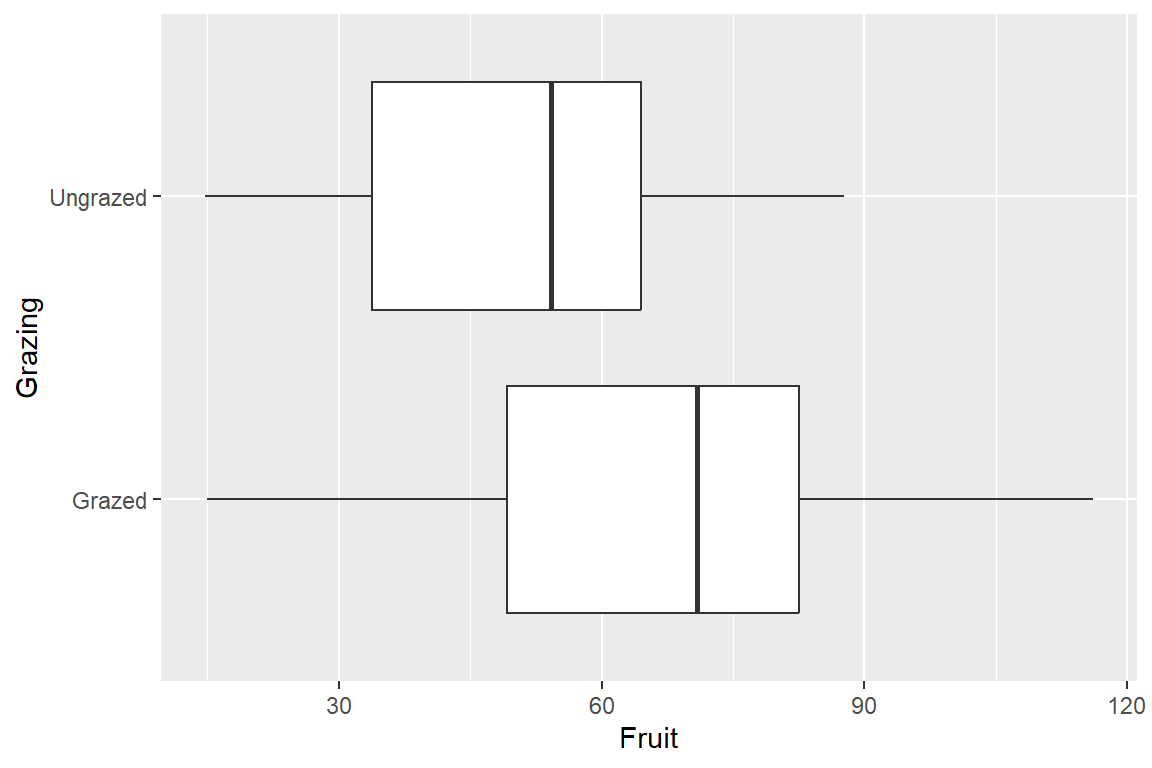
# Hypothesis test
t.test(Fruit ~ Grazing, data = df1, alternative = c("greater"))
    Welch Two Sample t-test

data:  Fruit by Grazing
t = 2.304, df = 37.306, p-value = 0.01344
alternative hypothesis: true difference in means between group Grazed and group Ungrazed is greater than 0
95 percent confidence interval:
 4.570757      Inf
sample estimates:
  mean in group Grazed mean in group Ungrazed
               67.9405                50.8805
Example 2: What is the influence of grazing and root diameter on the fruit production of a plant?
Independent variables:
- grazing (categorical: grazed or ungrazed)
- root diameter (continuous, mm, covariate)
Dependent variable:
- fruit production (mg)
# Visualization
ggplot(df1, aes(Root, Fruit))+
  geom_point() +
  geom_smooth(method = 'lm') +
  geom_point(aes(color = Grazing)) +
  geom_smooth(aes(color = Grazing), method = 'lm')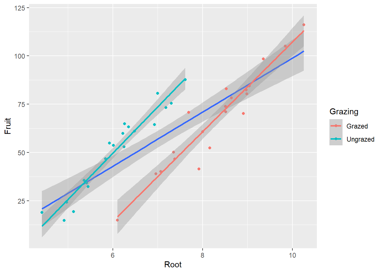
9.2.2 Maximal model
| Symbol | Meaning |
|---|---|
~ |
Separating DV (left) and IV (right) |
: |
Interaction effect of two factors |
* |
Main effect of the two factors and the interaction effect. f1 * f2 is equivalent to f1 + f2 + f1:f2 |
^ |
Square the sum of several terms. The main effect of these terms and the interaction between them |
. |
All variables except the DV |
# The maximal model
df1_ancova <- lm(Fruit ~ Grazing * Root, data = df1)
summary(df1_ancova)
Call:
lm(formula = Fruit ~ Grazing * Root, data = df1)

Residuals:
     Min       1Q   Median       3Q      Max
-17.3177  -2.8320   0.1247   3.8511  17.1313

Coefficients:
                     Estimate Std. Error t value Pr(>|t|)
(Intercept)          -125.173     12.811  -9.771 1.15e-11 ***
GrazingUngrazed        30.806     16.842   1.829   0.0757 .
Root                   23.240      1.531  15.182  < 2e-16 ***
GrazingUngrazed:Root    0.756      2.354   0.321   0.7500
---
Signif. codes:  0 '***' 0.001 '**' 0.01 '*' 0.05 '.' 0.1 ' ' 1

Residual standard error: 6.831 on 36 degrees of freedom
Multiple R-squared:  0.9293,    Adjusted R-squared:  0.9234
F-statistic: 157.6 on 3 and 36 DF,  p-value: < 2.2e-16
# The ANOVA table for the maximal model
anova(df1_ancova)Analysis of Variance Table
Response: Fruit
Df Sum Sq Mean Sq F value Pr(>F)
Grazing 1 2910.4 2910.4 62.3795 2.262e-09 ***
Root 1 19148.9 19148.9 410.4201 < 2.2e-16 ***
Grazing:Root 1 4.8 4.8 0.1031 0.75
Residuals 36 1679.6 46.7
---
Signif. codes: 0 '***' 0.001 '**' 0.01 '*' 0.05 '.' 0.1 ' ' 1# other method to see the ANOVA table
df1_aov <- aov(Fruit ~ Grazing * Root, data = df1)
summary(df1_aov) Df Sum Sq Mean Sq F value Pr(>F)
Grazing 1 2910 2910 62.380 2.26e-09 ***
Root 1 19149 19149 410.420 < 2e-16 ***
Grazing:Root 1 5 5 0.103 0.75
Residuals 36 1680 47
---
Signif. codes: 0 '***' 0.001 '**' 0.01 '*' 0.05 '.' 0.1 ' ' 1summary.aov(df1_ancova) Df Sum Sq Mean Sq F value Pr(>F)
Grazing 1 2910 2910 62.380 2.26e-09 ***
Root 1 19149 19149 410.420 < 2e-16 ***
Grazing:Root 1 5 5 0.103 0.75
Residuals 36 1680 47
---
Signif. codes: 0 '***' 0.001 '**' 0.01 '*' 0.05 '.' 0.1 ' ' 19.2.3 Minimal model
# Delete the interaction factor
df1_ancova2 <- update(df1_ancova, ~ . - Grazing:Root)
summary(df1_ancova2)
Call:
lm(formula = Fruit ~ Grazing + Root, data = df1)

Residuals:
     Min       1Q   Median       3Q      Max
-17.1920  -2.8224   0.3223   3.9144  17.3290

Coefficients:
                Estimate Std. Error t value Pr(>|t|)
(Intercept)     -127.829      9.664  -13.23 1.35e-15 ***
GrazingUngrazed   36.103      3.357   10.75 6.11e-13 ***
Root              23.560      1.149   20.51  < 2e-16 ***
---
Signif. codes:  0 '***' 0.001 '**' 0.01 '*' 0.05 '.' 0.1 ' ' 1

Residual standard error: 6.747 on 37 degrees of freedom
Multiple R-squared:  0.9291,    Adjusted R-squared:  0.9252
F-statistic: 242.3 on 2 and 37 DF,  p-value: < 2.2e-16
# Compare the simplified model with the maximal model
anova(df1_ancova, df1_ancova2)Analysis of Variance Table
Model 1: Fruit ~ Grazing * Root
Model 2: Fruit ~ Grazing + Root
Res.Df RSS Df Sum of Sq F Pr(>F)
1 36 1679.7
2 37 1684.5 -1 -4.8122 0.1031 0.75# Delete the grazing factor
df1_ancova3 <- update(df1_ancova2, ~ . - Grazing)
summary(df1_ancova3)
Call:
lm(formula = Fruit ~ Root, data = df1)

Residuals:
     Min       1Q   Median       3Q      Max
-29.3844 -10.4447  -0.7574  10.7606  23.7556

Coefficients:
            Estimate Std. Error t value Pr(>|t|)
(Intercept)  -41.286     10.723  -3.850 0.000439 ***
Root          14.022      1.463   9.584  1.1e-11 ***
---
Signif. codes:  0 '***' 0.001 '**' 0.01 '*' 0.05 '.' 0.1 ' ' 1

Residual standard error: 13.52 on 38 degrees of freedom
Multiple R-squared:  0.7073,    Adjusted R-squared:  0.6996
F-statistic: 91.84 on 1 and 38 DF,  p-value: 1.099e-11
# Compare the two models
anova(df1_ancova2, df1_ancova3)Analysis of Variance Table
Model 1: Fruit ~ Grazing + Root
Model 2: Fruit ~ Root
Res.Df RSS Df Sum of Sq F Pr(>F)
1 37 1684.5
2 38 6948.8 -1 -5264.4 115.63 6.107e-13 ***
---
Signif. codes: 0 '***' 0.001 '**' 0.01 '*' 0.05 '.' 0.1 ' ' 1summary(df1_ancova2)
Call:
lm(formula = Fruit ~ Grazing + Root, data = df1)

Residuals:
     Min       1Q   Median       3Q      Max
-17.1920  -2.8224   0.3223   3.9144  17.3290

Coefficients:
                Estimate Std. Error t value Pr(>|t|)
(Intercept)     -127.829      9.664  -13.23 1.35e-15 ***
GrazingUngrazed   36.103      3.357   10.75 6.11e-13 ***
Root              23.560      1.149   20.51  < 2e-16 ***
---
Signif. codes:  0 '***' 0.001 '**' 0.01 '*' 0.05 '.' 0.1 ' ' 1

Residual standard error: 6.747 on 37 degrees of freedom
Multiple R-squared:  0.9291,    Adjusted R-squared:  0.9252
F-statistic: 242.3 on 2 and 37 DF, p-value: < 2.2e-16anova(df1_ancova2)Analysis of Variance Table
Response: Fruit
Df Sum Sq Mean Sq F value Pr(>F)
Grazing 1 2910.4 2910.4 63.929 1.397e-09 ***
Root 1 19148.9 19148.9 420.616 < 2.2e-16 ***
Residuals 37 1684.5 45.5
---
Signif. codes: 0 '***' 0.001 '**' 0.01 '*' 0.05 '.' 0.1 ' ' 19.2.4 One step
Criterion: Akaike’s information criterion (AIC). The model is worse if AIC gets greater.
step(df1_ancova)Start: AIC=157.5
Fruit ~ Grazing * Root
Df Sum of Sq RSS AIC
- Grazing:Root 1 4.8122 1684.5 155.61
<none> 1679.7 157.50
Step: AIC=155.61
Fruit ~ Grazing + Root
Df Sum of Sq RSS AIC
<none> 1684.5 155.61
- Grazing 1 5264.4 6948.8 210.30
- Root 1 19148.9 20833.4 254.22
Call:
lm(formula = Fruit ~ Grazing + Root, data = df1)

Coefficients:
    (Intercept)  GrazingUngrazed             Root
        -127.83            36.10            23.56
9.2.5 Result
# Extracting formulas from linear regression models
equatiomatic::extract_eq(df1_ancova2, use_coefs = TRUE)
\[ \operatorname{\widehat{Fruit}} = -127.83 + 36.1(\operatorname{Grazing}_{\operatorname{Ungrazed}}) + 23.56(\operatorname{Root}) \]
# Create a diagnostic statistical data text table
stargazer::stargazer(df1_ancova2, type = 'text')
===============================================
                        Dependent variable:
                    ---------------------------
                               Fruit
-----------------------------------------------
GrazingUngrazed              36.103***
                              (3.357)

Root                         23.560***
                              (1.149)

Constant                    -127.829***
                              (9.664)

-----------------------------------------------
Observations                    40
R2                             0.929
Adjusted R2                    0.925
Residual Std. Error       6.747 (df = 37)
F Statistic           242.272*** (df = 2; 37)
===============================================
Note:               *p<0.1; **p<0.05; ***p<0.01
The meaning of each parameter in this table
- Dependent variable: The name of the dependent variable. (因变量的名称)
- Independent variables: The names of the independent variables. (自变量的名称)
- Coefficients: Regression coefficients, indicating the degree to which an independent variable affects the dependent variable when it increases by one unit. (回归系数,表示自变量每增加一个单位对因变量的影响程度)
- Standard errors: Standard error of regression coefficients, measuring the stability of regression coefficients. (回归系数的标准误差,衡量回归系数的稳定性)
- t-statistics: t-value of regression coefficients, representing whether a regression coefficient is significantly different from zero and has a significant impact on the dependent variable. (回归系数的t值,代表回归系数是否显著不为0,即是否对因变量有显著影响)
- p-values: Significance level of regression coefficients, usually used to determine whether a regression coefficient is significantly different from zero. The smaller the p-value, the more significant the regression coefficient is considered to be. (回归系数的显著性水平,通常用于判断回归系数是否显著不为0,p值越小,表示回归系数越显著)
- Observations: Sample size. (样本数量)
- R2: Goodness-of-fit measure that represents how much variance in explanatory variables can be explained by model. A higher value indicates better fit between model and data. (拟合优度,表示模型解释变量方差的比例,数值越高表示模型拟合程度越好)
- Adjusted R2:A modified version of R2 that takes into account number of independent variables for greater accuracy. (调整后的拟合优度,考虑到自变量的个数,比R2更准确)
- Residual standard error:Standard deviation or dispersion measure for residuals; smaller values indicate better model fit. (残差标准误,表示残差的离散程度,越小表示模型越好)
- F-statistic:Statistical test used to evaluate overall goodness-of-fit for linear models. (F统计量,用于检验模型整体拟合优度是否显著)
- df:Degrees of freedom. (自由度)
- Note:p<0.1,p<0.05,p<0.01 : When p-value is less than 0.1, 0.05 or 0.01 respectively,* , ** , *** are used as symbols indicating significance levels for corresponding regressions coefficients. (p<0.1, p<0.05, p<0.01:p值小于0.1,0.05,0.01时,分别用,,表示,代表回归系数的显著性水平)
9.3 Two-way ANCOVA
9.3.1 Question
Previous experiments have shown that both genotype and sex of an organism affect body weight gain. However, a scientist believes that after adjusting for age, there was no significant difference in means of weight gain between groups at different levels of sex and Genotype. Can experiments support this claim?
- Independent variables:
- genotype (categorical)
- sex (categorical)
- age (covariate)
- Dependent variable:
- Weight gain (continuous)
9.3.2 Model
Gain <- read.table("data/Gain.txt", header = T)
head(Gain, 3)
Weight Sex Age Genotype Score
1 7.445630 male 1 CloneA 4
2 8.000223 male 2 CloneA 4
3 7.705105 male 3 CloneA 4m1 <- lm(Weight ~ Sex * Age * Genotype, data = Gain)
summary(m1)
Call:
lm(formula = Weight ~ Sex * Age * Genotype, data = Gain)

Residuals:
     Min       1Q   Median       3Q      Max
-0.40218 -0.12043 -0.01065  0.12592  0.44687

Coefficients:
                           Estimate Std. Error t value Pr(>|t|)
(Intercept)                 7.80053    0.24941  31.276  < 2e-16 ***
Sexmale                    -0.51966    0.35272  -1.473  0.14936
Age                         0.34950    0.07520   4.648 4.39e-05 ***
GenotypeCloneB              1.19870    0.35272   3.398  0.00167 **
GenotypeCloneC             -0.41751    0.35272  -1.184  0.24429
GenotypeCloneD              0.95600    0.35272   2.710  0.01023 *
GenotypeCloneE             -0.81604    0.35272  -2.314  0.02651 *
GenotypeCloneF              1.66851    0.35272   4.730 3.41e-05 ***
Sexmale:Age                -0.11283    0.10635  -1.061  0.29579
Sexmale:GenotypeCloneB     -0.31716    0.49882  -0.636  0.52891
Sexmale:GenotypeCloneC     -1.06234    0.49882  -2.130  0.04010 *
Sexmale:GenotypeCloneD     -0.73547    0.49882  -1.474  0.14906
Sexmale:GenotypeCloneE     -0.28533    0.49882  -0.572  0.57087
Sexmale:GenotypeCloneF     -0.19839    0.49882  -0.398  0.69319
Age:GenotypeCloneB         -0.10146    0.10635  -0.954  0.34643
Age:GenotypeCloneC         -0.20825    0.10635  -1.958  0.05799 .
Age:GenotypeCloneD         -0.01757    0.10635  -0.165  0.86970
Age:GenotypeCloneE         -0.03825    0.10635  -0.360  0.72123
Age:GenotypeCloneF         -0.05512    0.10635  -0.518  0.60743
Sexmale:Age:GenotypeCloneB  0.15469    0.15040   1.029  0.31055
Sexmale:Age:GenotypeCloneC  0.35322    0.15040   2.349  0.02446 *
Sexmale:Age:GenotypeCloneD  0.19227    0.15040   1.278  0.20929
Sexmale:Age:GenotypeCloneE  0.13203    0.15040   0.878  0.38585
Sexmale:Age:GenotypeCloneF  0.08709    0.15040   0.579  0.56616
---
Signif. codes:  0 '***' 0.001 '**' 0.01 '*' 0.05 '.' 0.1 ' ' 1

Residual standard error: 0.2378 on 36 degrees of freedom
Multiple R-squared:  0.9742,    Adjusted R-squared:  0.9577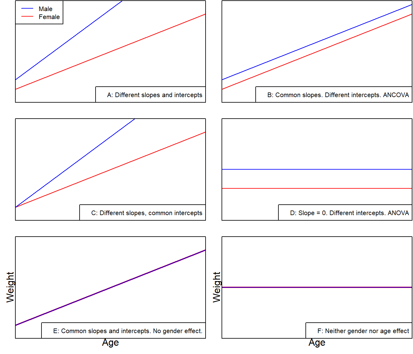
F-statistic: 59.06 on 23 and 36 DF, p-value: < 2.2e-16- There are no things like Age:Sex or Age:Genotype, so the slope of weight gain against age does not vary with sex or genotype
- In the final minimal adequate model, three main effects were included (Sex, Age, Genotype), so it can be considered that there are intercept differences between gender, age and genotype (intercepts vary).
- The final minimal adequate model includes three main effects (Sex, Age, Genotype), but no interaction effect. This means that the effects of these variables are independent and there is no interaction between them.
9.3.3 One step
m2 <- step(m1)Start: AIC=-155.01
Weight ~ Sex * Age * Genotype
Df Sum of Sq RSS AIC
- Sex:Age:Genotype 5 0.34912 2.3849 -155.51
<none> 2.0358 -155.01
Step: AIC=-155.51
Weight ~ Sex + Age + Genotype + Sex:Age + Sex:Genotype + Age:Genotype
Df Sum of Sq RSS AIC
- Sex:Genotype 5 0.146901 2.5318 -161.92
- Age:Genotype 5 0.168136 2.5531 -161.42
- Sex:Age 1 0.048937 2.4339 -156.29
<none> 2.3849 -155.51
Step: AIC=-161.92
Weight ~ Sex + Age + Genotype + Sex:Age + Age:Genotype
Df Sum of Sq RSS AIC
- Age:Genotype 5 0.168136 2.7000 -168.07
- Sex:Age 1 0.048937 2.5808 -162.78
<none> 2.5318 -161.92
Step: AIC=-168.07
Weight ~ Sex + Age + Genotype + Sex:Age
Df Sum of Sq RSS AIC
- Sex:Age 1 0.049 2.749 -168.989
<none> 2.700 -168.066
- Genotype 5 54.958 57.658 5.612
Step: AIC=-168.99
Weight ~ Sex + Age + Genotype
Df Sum of Sq RSS AIC
<none> 2.749 -168.989
- Sex 1 10.374 13.122 -77.201
- Age 1 10.770 13.519 -75.415
- Genotype 5 54.958 57.707 3.662summary(m2)
Call:
lm(formula = Weight ~ Sex + Age + Genotype, data = Gain)

Residuals:
     Min       1Q   Median       3Q      Max
-0.40005 -0.15120 -0.01668  0.16953  0.49227

Coefficients:
               Estimate Std. Error t value Pr(>|t|)
(Intercept)     7.93701    0.10066  78.851  < 2e-16 ***
Sexmale        -0.83161    0.05937 -14.008  < 2e-16 ***
Age             0.29958    0.02099  14.273  < 2e-16 ***
GenotypeCloneB  0.96778    0.10282   9.412 8.07e-13 ***
GenotypeCloneC -1.04361    0.10282 -10.149 6.21e-14 ***
GenotypeCloneD  0.82396    0.10282   8.013 1.21e-10 ***
GenotypeCloneE -0.87540    0.10282  -8.514 1.98e-11 ***
GenotypeCloneF  1.53460    0.10282  14.925  < 2e-16 ***
---
Signif. codes:  0 '***' 0.001 '**' 0.01 '*' 0.05 '.' 0.1 ' ' 1

Residual standard error: 0.2299 on 52 degrees of freedom
Multiple R-squared:  0.9651,    Adjusted R-squared:  0.9604
F-statistic: 205.7 on 7 and 52 DF,  p-value: < 2.2e-16
From the above output, we can see the coefficients of each genotype and their corresponding significance level (in the Estimate column). It can be observed that GenotypeCloneC and GenotypeCloneE have similar effects on the dependent variable, with coefficients close to -1 and very small significance levels (p-value < 0.001). Therefore, we can combine these two factors into one factor, reducing the number of genotype levels from six to five. The same approach can be applied to B and D.
# Check
newGenotype <- as.factor(Gain$Genotype)
levels(newGenotype)
[1] "CloneA" "CloneB" "CloneC" "CloneD" "CloneE" "CloneF"# Change
levels(newGenotype)[c(3,5)] <- "ClonesCandE"
levels(newGenotype)[c(2,4)] <- "ClonesBandD"
levels(newGenotype)[1] "CloneA" "ClonesBandD" "ClonesCandE" "CloneF" # Liner regression & compare
m3 <- lm(Weight ~ Sex + Age + newGenotype, data = Gain)
anova(m2,m3)Analysis of Variance Table
Model 1: Weight ~ Sex + Age + Genotype
Model 2: Weight ~ Sex + Age + newGenotype
Res.Df RSS Df Sum of Sq F Pr(>F)
1 52 2.7489
2 54 2.9938 -2 -0.24489 2.3163 0.1087Analysis of RSS above
In regression models, the residual sum of squares (RSS) represents the unexplained variance in the dependent variable. In this example, the RSS for Model 1 and Model 2 are 2.7489 and 2.9938 respectively. The goal of a model is to minimize RSS because it represents how well the model fits with observed values. Generally, a smaller RSS indicates a better fit for the model. When comparing two models’ fit, one can use both RSS and F-statistic. In this example, although Model 2 has a slightly larger RSS than Model 1, its P-value for F-statistic is 0.1087 which does not reach commonly used significance levels such as 0.05; therefore we cannot reject null hypothesis that Model 2 performs worse than Model 1.9.3.4 Result
As \(p=0.1087\), there is no significant difference between the two models. Therefore, the new model uses NewGenotype (four levels) instead of Genotype (six levels).
summary(m3)
Call:
lm(formula = Weight ~ Sex + Age + newGenotype, data = Gain)
Residuals:
Min 1Q Median 3Q Max
-0.42651 -0.16687 0.01211 0.18776 0.47736
Coefficients:
Estimate Std. Error t value Pr(>|t|)
(Intercept) 7.93701 0.10308 76.996 < 2e-16 ***
Sexmale -0.83161 0.06080 -13.679 < 2e-16 ***
Age 0.29958 0.02149 13.938 < 2e-16 ***
newGenotypeClonesBandD 0.89587 0.09119 9.824 1.28e-13 ***
newGenotypeClonesCandE -0.95950 0.09119 -10.522 1.10e-14 ***
newGenotypeCloneF 1.53460 0.10530 14.574 < 2e-16 ***
---
Signif. codes: 0 '***' 0.001 '**' 0.01 '*' 0.05 '.' 0.1 ' ' 1
Residual standard error: 0.2355 on 54 degrees of freedom
Multiple R-squared: 0.962, Adjusted R-squared: 0.9585
F-statistic: 273.7 on 5 and 54 DF, p-value: < 2.2e-16# Extracting formulas from linear regression models
equatiomatic::extract_eq(m3, use_coefs = TRUE)\[ \operatorname{\widehat{Weight}} = 7.94 - 0.83(\operatorname{Sex}_{\operatorname{male}}) + 0.3(\operatorname{Age}) + 0.9(\operatorname{newGenotype}_{\operatorname{ClonesBandD}}) - 0.96(\operatorname{newGenotype}_{\operatorname{ClonesCandE}}) + 1.53(\operatorname{newGenotype}_{\operatorname{CloneF}}) \]
# Create a diagnostic statistical data text table
stargazer::stargazer(m3, type = 'text')
==================================================
Dependent variable:
---------------------------
Weight
--------------------------------------------------
Sexmale -0.832***
(0.061)
Age 0.300***
(0.021)
newGenotypeClonesBandD 0.896***
(0.091)
newGenotypeClonesCandE -0.960***
(0.091)
newGenotypeCloneF 1.535***
(0.105)
Constant 7.937***
(0.103)
--------------------------------------------------
Observations 60
R2 0.962
Adjusted R2 0.959
Residual Std. Error 0.235 (df = 54)
F Statistic 273.652*** (df = 5; 54)
==================================================
Note: *p<0.1; **p<0.05; ***p<0.019.3.5 Visualization
plot(Weight~Age,data=Gain,type="n")
colours <- c("green","red","black","blue")
lines <- c(1,2)
symbols <- c(16,17)
NewSex<-as.factor(Gain$Sex)
points(Weight~Age,data=Gain,pch=symbols[as.numeric(NewSex)],
col=colours[as.numeric(newGenotype)])
xv <- c(1,5)
for (i in 1:2) {
for (j in 1:4){
a <- coef(m3)[1]+(i>1)* coef(m3)[2]+(j>1)*coef(m3)[j+2]
b <- coef(m3)[3]
yv <- a+b*xv
lines(xv,yv,lty=lines[i],col=colours[j]) } }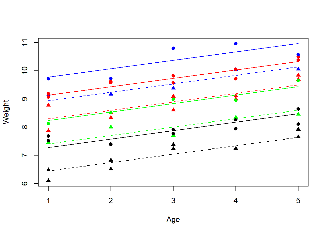
10 MANCOVA

- Dependent variables: multiple continuous variables
- Independent variables: one or multiple categorical variables, one or multiple continuous variables (covariates)
10.1 Definition of MANCOVA
Multivariate Analysis of Covariance (MANCOVA) = multivariate ANCOVA = MANOVA with covariate(s)
Analysis for the differences among group means for a linear combination of the dependent variables after adjusted for the covariate. Test whether the independent variable(s) has a significant influence on the dependent variables, excluding the influence of the covariate (preferably highly correlated with the dependent variable)
- Independent Random Sampling: Independence of observations from all other observations.
- Level and Measurement of the Variables: The independent variables are categorical and the dependent variables are continuous or scale variables. Covariates are continuous.
- Homogeneity of Variance: Variance between groups is equal.
- Normality: For each group, each dependent variable follows a normal distribution and any linear combination of dependent variables are normally distributed
Brief explanation in Chinese
在MANCOVA中,我们有多个因变量(即连续或比例变量),一个或多个自变量(即分类变量),以及一个或多个协变量(即连续变量)。这些变量的测量水平应该正确,并且观察值应该是独立随机采样的。这意味着,我们要确保观察值彼此独立,不受其他变量的影响。同时,我们需要检查每个组的因变量是否都符合正态分布,并且方差应该相等。如果我们的数据满足这些假设,则可以使用MANCOVA来探索自变量对因变量的影响,并且通过协变量来控制一些其他影响因素的影响。MANCOVA可以更准确地确定组间差异是否真实存在,而不是基于单个因变量的分析来做出判断。 MANCOVA通常用于实验设计,研究人员想要比较多个组的平均得分,同时控制其他因素的影响。
10.2 Workflow
10.2.1 Question
Example: Are there differences in productivity (measured by income and hours worked) for individuals in different age groups after adjusted for the education level?
- Dependent variables:
- wage (continuous)
- age (continuous)
- Independent variables:
- education (categorical)
- year (continuous, covariate)
10.2.2 Visualization
library(tidyverse)
library(ISLR)
library(car)
ggplot(Wage, aes(age, wage)) + geom_point(alpha = 0.3) +
geom_smooth(method = lm) + facet_grid(year~education)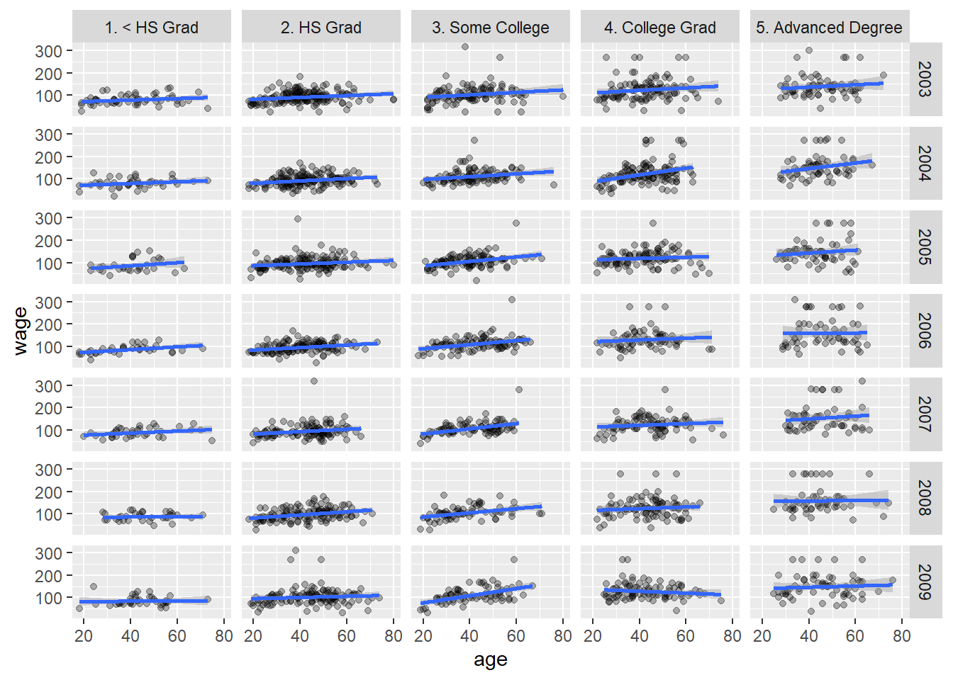
10.2.3 Model
manova()way
wage_manova1 <- manova(cbind(wage, age) ~ education * year, data = Wage)
wage_manova1Call:
manova(cbind(wage, age) ~ education * year, data = Wage)
Terms:
education year education:year Residuals
wage 1226364 16807 2404 3976510
age 4608 494 724 393723
Deg. of Freedom 4 1 4 2990
Residual standard errors: 36.4683 11.47519
Estimated effects may be unbalancedsummary.aov(wage_manova1) Response wage :
Df Sum Sq Mean Sq F value Pr(>F)
education 4 1226364 306591 230.5306 < 2.2e-16 ***
year 1 16807 16807 12.6374 0.000384 ***
education:year 4 2404 601 0.4519 0.771086
Residuals 2990 3976510 1330
---
Signif. codes: 0 '***' 0.001 '**' 0.01 '*' 0.05 '.' 0.1 ' ' 1
Response age :
Df Sum Sq Mean Sq F value Pr(>F)
education 4 4608 1151.90 8.7477 5.108e-07 ***
year 1 494 494.13 3.7525 0.05282 .
education:year 4 724 180.90 1.3738 0.24043
Residuals 2990 393723 131.68
---
Signif. codes: 0 '***' 0.001 '**' 0.01 '*' 0.05 '.' 0.1 ' ' 1Brief explanation in Chinese
根据结果,教育和年份两个因子对 wage 有显著影响,因为它们的 P 值均小于0.05。但是,交互作用项 “education:year” 的 P 值大于0.05,表明这个交互项对 wage 没有显著影响。对于年龄变量,教育和(年份≈0.05)都对其有显著影响,因为它们的 P 值小于0.05。然而,交互项 “education:year” 对 age 没有显著影响,因为其 P 值大于0.05。
jmv::mancova()way
library(jmv)
wage_manova2 <- jmv::mancova(data = Wage,
deps = vars(wage, age),
factors = education,
covs = year)
wage_manova2
MANCOVA
Multivariate Tests
─────────────────────────────────────────────────────────────────────────────────────────────
value F df1 df2 p
─────────────────────────────────────────────────────────────────────────────────────────────
education Pillai's Trace 0.240590546 102.353675 8 5988 < .0000001
Wilks' Lambda 0.7605539 109.739015 8 5986 < .0000001
Hotelling's Trace 0.313326457 117.184095 8 5984 < .0000001
Roy's Largest Root 0.308447997 230.873326 4 2994 < .0000001
year Pillai's Trace 0.004790217 7.203065 2 2993 0.0007573
Wilks' Lambda 0.9952098 7.203065 2 2993 0.0007573
Hotelling's Trace 0.004813274 7.203065 2 2993 0.0007573
Roy's Largest Root 0.004813274 7.203065 2 2993 0.0007573
─────────────────────────────────────────────────────────────────────────────────────────────
Univariate Tests
────────────────────────────────────────────────────────────────────────────────────────────────────────
Dependent Variable Sum of Squares df Mean Square F p
────────────────────────────────────────────────────────────────────────────────────────────────────────
education wage 1226364.4849 4 306591.1212 230.699570 < .0000001
age 4607.5852 4 1151.8963 8.743336 0.0000005
year wage 16806.9907 1 16806.9907 12.646699 0.0003821
age 494.1336 1 494.1336 3.750664 0.0528805
Residuals wage 3978914.2941 2994 1328.9627
age 394446.4359 2994 131.7456
──────────────────────────────────────────────────────────────────────────────────────────────────────── Brief explanation in Chinese
在 Multivariate Tests 表格中,我们可以看到 education 和 year 这两个自变量的多元假设检验结果。四种统计量都显示了这两个变量的组合对因变量 wage 和 age 有显著影响(p 值 < 0.0001)。在 Univariate Tests 表格中,我们可以看到每个因变量 wage 和 age 的单元假设检验结果。结果显示 education 对 wage 和 age 都有显著影响(p 值 < 0.0001),而 year 只对 wage 有显著影响(p 值 = 0.0004)。值得注意的是,age 的 year 效应在 p 值为 0.0529 的边缘。Residuals 列显示了每个因变量在模型中的残差方差。
总体来说,这个 MANCOVA 模型表明,在控制了 education 和 year 之后,wage 和 age 之间存在着相关性,并且 education 和 year 对这种关系都有显著的影响。
10.2.4 Result
- Since the interaction effect is not significant (p = 0.77 for salary and p = 0.24 for age), the slopes are parallel.
- The wage and age differ significantly among education groups (p for both wage and age are far below 0.05).
- Differences in salary also significantly (p = 0.00038) increase over time (variable year), due to some economic reasons, while differences in age don’t change (p = 0.053) much.
Brief explanation in Chinese
- 对于交互作用效应而言,它在wage和age方面的p值分别为0.771086和0.24043,因此交互作用效应不显著。这意味着不同教育水平组之间的工资和年龄差异的斜率是平行的。
- 对于MANOVA表格中的“Multivariate Tests”部分,education组之间的差异在wage和age方面都显著(p值均远远低于0.05)。
- 对于ANOVA表格中的“Univariate Tests”部分,随时间的推移,salary方面的差异显著增加(p=0.000384),而age方面的差异则没有显著变化(p=0.05282)。这表明时间变化是造成salary变化的一个重要原因,而不是年龄变化。
11 Combining statistics
11.1 Combining means and standard errors
Example: Two separate but similar experiments measuring the rate of glucose production of liver cells.
Tips: for different group experments we can’t just sum them up and simply calculate the mean and standard error.
- Experiment 1: 4.802, 3.81, 4.004, 4.467, 3.8
- Experiment 2: 5.404, 5.256, 4.145, 5.401, 5.622, 4.312
- Calculate the overall \(n, \bar x, se\)
If we know the row data:
# Row data
x1 <- c(4.802, 3.81, 4.004, 4.467, 3.8)
x2 <- c(5.404, 5.256, 4.145, 5.401, 5.622, 4.312)
# Form a new dataframe which contains Those columns
n1 <- length(x1)
n2 <- length(x2)
dtf <- data.frame(n = c(n1, n2), mean = c(mean(x1), mean(x2)), sd = c(sd(x1), sd(x2)))
dtf$se <- dtf$sd/sqrt(dtf$n)
dtf n mean sd se
1 5 4.176600 0.4420043 0.1976703
2 6 5.023333 0.6288942 0.2567450# Calculate the mean and standard error
x <- c(x1, x2)
x_bar <- mean(x)
n <- length(x)
se <- sd(x)/sqrt(n)
c(x_bar, se)[1] 4.6384545 0.2070211If we don’t know the row data:
cmean <- sum(dtf$mean * dtf$n) / sum(dtf$n)
cse <- sqrt((sum(dtf$n * ((dtf$n - 1)* dtf$se ^ 2 + dtf$mean ^ 2)) - sum(dtf$n * dtf$mean) ^ 2/ sum(dtf$n)) / (sum(dtf$n) * (sum(dtf$n) - 1)))
c(cmean, cse)[1] 4.6384545 0.207021111.2 Mean and standard errors of sum and difference
11.2.1 Concepts
- First we have two variables \(p\) and \(q\)
- The third variable \(x = p + q\)
- The fourth variable \(y = p - q\)
- When \(n_p \neq n_q \neq n\): \[\bar x = \bar p + \bar q\] \[\bar y = \bar p - \bar q\] \[se_x = se_y = \sqrt{\frac{(n_p - 1)se_p^2 + (n_q - 1)se_q^2}{n_p + n_q - 2} \cdot \frac{n_p + n_q}{n_p n_q}}\]
- When \(n_p = n_q = n\): \[se_x = se_y = \sqrt{\frac{se_p^2 + se_q^2}{n}}\]
11.2.2 Example
A luciferase-based assay is being used to quantify the amount of ATP and ADP in small tissue samples. The amount of ATP (q) is measured directly in 8 samples as \(3.25 \pm 0.14 mol g^{-1}\). A further 10 samples are treated with pyruvate kinase plus phosphoenolpyruvate to convert ADP quantitatively to ATP. The total ATP (p) in these samples is determined to be \(4.56 \pm 0.29\mu mol g^{-1}\). The ADP content is \(p - q\).
What is the mean and standard error of ADP concentration?
# Dataframe of example experiment
x <- data.frame(mean = c(3.25, 4.56), n = c(8, 10), se = c(0.14, 0.29))
x mean n se
1 3.25 8 0.14
2 4.56 10 0.29ADP <- diff(x$mean)
cse <- sqrt(sum(x$se ^ 2 * (x$n - 1)) / (sum(x$n) - 2) * sum(x$n) / prod(x$n))
c(ADP, cse)[1] 1.3100000 0.112130611.3 Mean and standard error of ratios and products
11.3.1 Concepts
- First we have two variables \(p\) and \(q\)
- The third variable \(x = p \cdot q\)
- The fourth variable \(y = p / q\) \[\bar x = \bar p \cdot \bar q\] \[\bar y = \bar p / \bar q\] \[se_x = \sqrt{\frac{\bar p^2 n_q se_q^2 + \bar q^2 n_p se_p^2 + n_p se_p^2 n_q se_q^2}{n_p + n_q - 2}}\] \[se_y = \frac{1}{\bar q} \sqrt {\frac{n_p se_p^2 + n_qse_q^2(\frac{\bar p}{\bar q})^2}{n_p + n_q - 2}}\]
11.3.2 Example
In the previous example, we got the concentrations of ATP and ADP in a tissue sample. what is the ratio of [ATP]/[ADP]?
x <- data.frame(mean = c(3.25, ADP), n = c(8, 10), se = c(0.14, cse))
x mean n se
1 3.25 8 0.1400000
2 1.31 10 0.1121306ratiox <- x$mean[1] / x$mean[2]
cse <- sqrt((x$n[1] * x$se[1] ^ 2 + x$n[2] * x$se[2] ^ 2 * ((x$mean[1] / x$mean[2]) ^ 2)) / (sum(x$n) - 2)) / x$mean[2]
c(ratiox, cse)[1] 2.4809160 0.184106312 Non-parametric hypothesis tests
12.1 Definition
Non-parametric hypothesis tests:
A hypothesis test that does not require any specific conditions concerning the shapes of population distributions or the values of population parameters. When we don’t know the distribution of the population, the it is easier to perform than corresponding parametric tests but less efficient than parametric tests.
Wilcoxon Rank-Sum test: Used to compare whether the medians of two independent groups are equal. It is suitable for situations where the sample does not follow a normal distribution or where the variances are unequal.
Wilcoxon Signed-Rank test: Used to compare whether the medians of two related groups are equal. It is suitable for situations where the sample does not follow a normal distribution or where the variances are unequal.
Kruskal-Wallis test: Used to compare whether the medians of three or more independent groups are equal. It is suitable for situations where the sample does not follow a normal distribution or where the variances are unequal.
Friedman test: Used to compare whether the medians of three or more related groups are equal. It is suitable for situations where the sample does not follow a normal distribution or where the variances are unequal.
12.2 Wilcoxon Rank-Sum test
12.2.1 Concept
Wilcoxon Rank-Sum test, also known as the Mann-Whitney U test, is a non-parametric test for comparing the equality of the medians of two independent samples. Its original hypothesis is that the medians of the two samples are equal, and the alternative hypothesis is that the medians of the two samples are not equal.
- \(H_0\): the medians of the two populations are equal.
- Both samples are drawn randomly and independently.
- The measures within the two samples are able to be ranked and hence must be continuous, discrete or ordinal.
The basic idea of this test is to combine the two samples, rank them in order of size, and then calculate how many of the rankings in each sample are less than or equal to the value of that sample. The sum of these rankings is then used as the test statistic. If the medians of the two samples are equal, the test statistic should be close to half the sum of the total rankings. If the medians of the two samples are not equal, then the test statistic should be far from half the sum of the total rankings. \[U=\sum_{i=1}^n \sum_{j=1}^m S\left(X_i, Y_j\right)\] \[S(X, Y)= \begin{cases}1, & \text { if } X>Y \\ \frac{1}{2}, & \text { if } X=Y \\ 0, & \text { if } X<Y\end{cases}\]
- \(U\): The Wilcoxon Rank-Sum test statistic
- \(X_1, \ldots, X_n\): an independent sample from \(X\)
- \(Y_1, \ldots, Y_m\): an independent sample from \(Y\)
12.2.2 Example-1
Suppose we have two dataset x and y, calculate the U (U is the smaller rank sum of these two samples):
# Row data
x <- c(3, 7)
y <- c(2, 4, 5, 8, 9)
m <- length(x)
n <- length(y)
# One step
# The outer() function is the function used in R to perform various operations between two vectors,
# returning the result of all operations between all elements of the two vectors.
U <- sum(outer(x, y, ">")) + sum(outer(x, y, "==")) * 0.5 + sum(outer(x, y, "<")) * 0
U[1] 4The larger of the m and n, the U more like normal distribution, approximately normal distribution by:
\[\mu_U = mn/2\] \[s_U = \sqrt{\frac{mn(m + n + 1)}{12}}\]
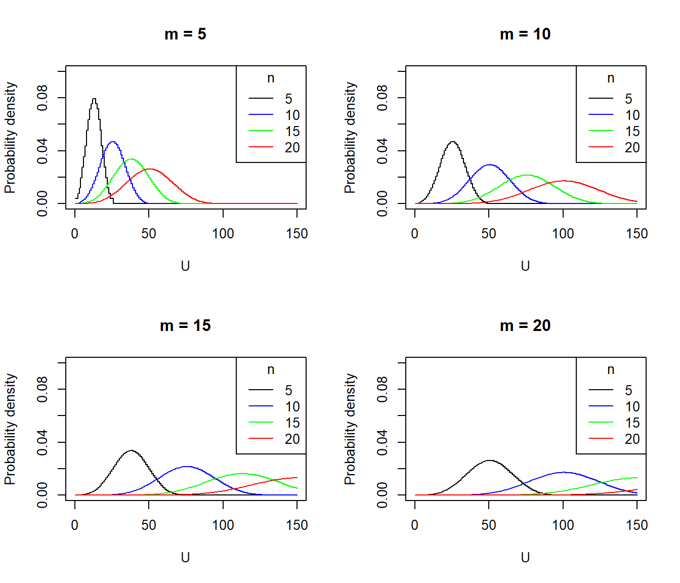
Ties concept:
# Duplicate value ranking
rank(c(1, 2, 2, 3))[1] 1.0 2.5 2.5 4.012.2.3 Workflow
# One step
wilcox.test(x, y)
Wilcoxon rank sum exact test
data: x and y
W = 4, p-value = 0.8571
alternative hypothesis: true location shift is not equal to 0dtf <- data.frame(value = c(x, y),
name = rep(c('x', 'y'), c(m, n)))
wilcox.test(value ~ name, data = dtf)
Wilcoxon rank sum exact test
data: value by name
W = 4, p-value = 0.8571
alternative hypothesis: true location shift is not equal to 0# Boxplot visualization
boxplot(x, y, horizontal = TRUE)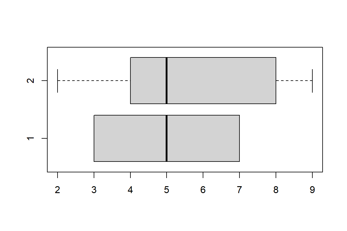
U_critical <- qwilcox(c(0.025, 0.975), m, n)
U_critical[1] 0 10pwilcox(U, m, n) * 2[1] 0.8571429# Probability density function plot visualization
curve(dwilcox(x, m, n), from = -1, to = 15, n = 17, ylab = 'Probability distribution density', las = 1, type = 'S', ylim = c(0, 0.15))
abline(h = 0)
segments(x0 = c(U, U_critical), y0 = 0, x1 = c(U, U_critical), y1 = dwilcox(c(U, U_critical), m, n), col = c('blue', 'red', 'red'))
legend('topright', legend = c('Distribution curve', 'Critical values', 'U score'), col = c('black', 'red', 'blue'), lty = 1, cex = 0.7)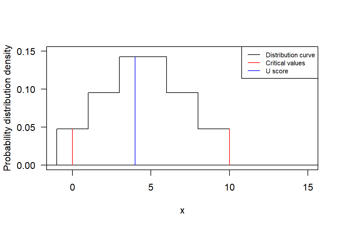
12.2.4 Example-2
The insect spray dataset for C, D and F (just the pick C and D). The number of insects that survived when treated with insecticide treatments.
# Row data
insect <- read.csv("data/InsectSprays.csv")
insect <- insect[insect$spray %in% c("C", "D"), ]
# Visualization
boxplot(bugs ~ spray, data = insect, horizontal = TRUE)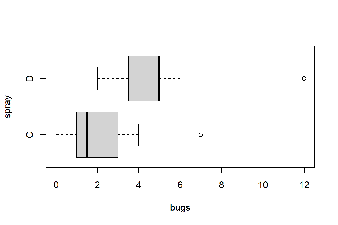
Use Shapiro test to test each of the group we treat to see if they are normal distribution:
shapiro.test(insect$bugs[insect$spray == "C"])
Shapiro-Wilk normality test
data: insect$bugs[insect$spray == "C"]
W = 0.85907, p-value = 0.04759shapiro.test(insect$bugs[insect$spray == "D"])
Shapiro-Wilk normality test
data: insect$bugs[insect$spray == "D"]
W = 0.75063, p-value = 0.002713Instead, we could test whether the two medians are different:
tapply(insect$bugs, insect$spray, median) C D
1.5 5.0 \(H_0\): The median of the survived insects treated by C is equal to that by D.
# Step by step
m <- sum(insect$spray == 'C')
n <- sum(insect$spray == 'D')
x <- insect$bugs[insect$spray == 'C']
y <- insect$bugs[insect$spray == 'D']
U1 <- sum(outer(x, y, ">")) + sum(outer(x, y, "==")) * 0.5
U2 <- sum(outer(y, x, ">")) + sum(outer(y, x, "==")) * 0.5
U <- min(c(U1, U2))
U_critical <- qwilcox(c(0.025, 0.975), m, n)
pwilcox(U, m, n) * 2[1] 0.001829776# Approximately z distribution
U_mu <- m * n / 2
U_sd <- sqrt(m * n * (m + n + 1) / 12)
z_score <- (U - U_mu)/U_sd
pnorm(z_score) * 2 [1] 0.002680172# Determine if there is a significant difference between those two sprays
median(outer(insect$bugs[insect$spray == 'C'], insect$bugs[insect$spray == 'D'], "-"))[1] -3# One step
wilcox.test(bugs ~ spray, data = insect, conf.int=TRUE)
Wilcoxon rank sum test with continuity correction
data: bugs by spray
W = 20, p-value = 0.002651
alternative hypothesis: true location shift is not equal to 0
95 percent confidence interval:
-4.000018 -1.000009
sample estimates:
difference in location
-2.999922 The meaning of each parameter in this table
- W: the Wilcoxon test statistic U.
- We are 95% certain that the median difference between spray D and C across the population will be between 1 and 4 bugs.
- It does not estimate the difference in medians but rather the median of the difference (between the two samples)
Decision: Reject \(H_0\)
Conclusion: There is a significant difference in insecticide effectiveness.
12.3 Wilcoxon Signed-Rank test
12.3.1 Concept
Test whether the median of the observed differences deviates enough from zero, based on paired samples. Roughly a non-parametric version of paired t-test.
\(H_0\): the medians of the two populations are equal.
12.3.2 Example
Ten people take part in a weight-loss program. They weigh before starting the program, and weigh again after the one-month program. Does the program have effect on the weight?
# Row data
wl <- data.frame(
id = LETTERS[1:10],
before = c(198, 201, 210, 185, 204, 156, 167, 197, 220, 186),
after = c(194, 203, 200, 183, 200, 153, 166, 197, 215, 184))
# Step by step
n <- nrow(wl)
d <- wl$after - wl$before
R <- rank(abs(d)) * abs(d) / d # signed ranks of the differences
W <- sum(R, na.rm = TRUE)
sW <- sqrt(n * (n + 1) * (2 * n + 1) / 6) # population standard deviation of W
z <- (abs(W) - 0.5) / sW
z_critical <- qnorm(p = c(0.025, 0.975)) # alpha = 0.05
pnorm(z, lower.tail = FALSE) * 2[1] 0.02040075# One step
wilcox.test(wl$before, wl$after, paired = TRUE, conf.int = TRUE, correct = FALSE)
Wilcoxon signed rank test
data: wl$before and wl$after
V = 42, p-value = 0.02032
alternative hypothesis: true location shift is not equal to 0
95 percent confidence interval:
0.9999463 6.0000301
sample estimates:
(pseudo)median
3.00007 Decision: As \(p < 0.05\), reject \(H_0\).
Conclusion: The two population medians are different at \(\alpha = 0.05\). The program has effect on the weight.
12.4 Kruskal-Wallis test
12.4.1 Concept
Test whether three or more population medians are equal. Roughly a non-parametric version of ANOVA
\(H_0\): the medians of the populations are equal.
12.4.2 Example
The insect spray dataset for C, D, and F. The number of insects that survived when treated with insecticide treatments.
Do any difference in the number of insects that survived when treated with multiple available insecticide treatments?
# Row data
insect <- read.csv("data/InsectSprays.csv")
# Visualization
boxplot(bugs ~ spray, data = insect, horizontal = TRUE, notch = TRUE)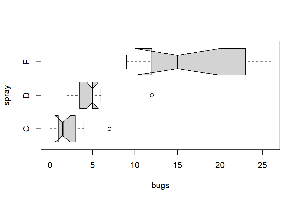
shapiro.test(insect$bugs[insect$spray == "C"]) # Normal distribution
Shapiro-Wilk normality test
data: insect$bugs[insect$spray == "C"]
W = 0.85907, p-value = 0.04759shapiro.test(insect$bugs[insect$spray == "D"]) # Normal distribution
Shapiro-Wilk normality test
data: insect$bugs[insect$spray == "D"]
W = 0.75063, p-value = 0.002713shapiro.test(insect$bugs[insect$spray == "F"]) # Not normal distribution
Shapiro-Wilk normality test
data: insect$bugs[insect$spray == "F"]
W = 0.88475, p-value = 0.1009# Determine if there is a significant difference between those three sprays
tapply(insect$bugs, insect$spray, median) C D F
1.5 5.0 15.0 # One step
kruskal.test(bugs ~ spray, data = insect)
Kruskal-Wallis rank sum test
data: bugs by spray
Kruskal-Wallis chi-squared = 26.866, df = 2, p-value = 1.466e-06Decision: As \(p < 0.05\), reject H0.
Conclusion: There is a significant difference in insecticide effectiveness.
12.5 Friedman’s test
12.5.1 Concept
Test whether three or more population medians are equal for repeated measures. Roughly a non-parametric version of repeated measures ANOVA. More powerful than ANOVA for very skewed (heavy tail) distributions. \[F_{r}=\frac{12}{n k(k+1)}\left(T_{1}^{2}+T_{2}^{2}+\ldots+T_{k}^{2}\right)-3 n(k+1)\]
12.5.2 Example
# Row data
dtf <- data.frame(
before = c(198, 201, 210, 185, 204, 156, 167, 197, 220, 186),
one = c(194, 203, 200, 183, 200, 153, 166, 197, 215, 184),
two = c(191, 200, 192, 180, 195, 150, 167, 195, 209, 179),
three = c(188, 196, 188, 178, 191, 145, 166, 192, 205, 175)
)
rownames(dtf) <- LETTERS[1:10]
k <- ncol(dtf)
n <- nrow(dtf)Calculate the Friedman test statistic:
# Rank of each group
dtf_rank <- t(apply(dtf, MARGIN = 1, rank))
dtf_rank before one two three
A 4.0 3.0 2.0 1.0
B 3.0 4.0 2.0 1.0
C 4.0 3.0 2.0 1.0
D 4.0 3.0 2.0 1.0
E 4.0 3.0 2.0 1.0
F 4.0 3.0 2.0 1.0
G 3.5 1.5 3.5 1.5
H 3.5 3.5 2.0 1.0
I 4.0 3.0 2.0 1.0
J 4.0 3.0 2.0 1.0# Method-1 of Chi-square value
rank_sum <- colSums(dtf_rank)
chi_sq <- 12 / (n * k * (k + 1)) * sum(rank_sum ^ 2) - 3 * n * (k + 1)
# Method-2 of Chi-square value
rank_mean <- colMeans(dtf_rank)
rank_overall <- mean(1:k)
ssb <- n * sum((rank_mean - rank_overall) ^ 2)
chi_sq <- 12 * ssb / (k * (k + 1))
chi_sq[1] 24.99# Critical point
chi_critical <- qchisq(0.05, df = k - 1, lower.tail = FALSE)
chi_critical[1] 7.814728# P-value
p_value <- pchisq(chi_sq, df = k - 1, lower.tail = FALSE)
p_value[1] 1.551501e-05# One step
friedman.test(as.matrix(dtf))
Friedman rank sum test
data: as.matrix(dtf)
Friedman chi-squared = 25.763, df = 3, p-value = 1.069e-05Tips: the sample is too small, so the results calculated manually may different from those using the R function which uses more accurate mathematical methods to calculate the value of the statistic.
13 Multiple linear regression
13.1 Definition
Linear Regression: A statistical method to determine the independent quantitative relationship between one or more predictor variables and one dependent variable.
- Simple Linear Regression: Only one predictor variable.
- Multiple linear regression: Two or more predictor variables.
Selection of predictor variables:
- The predictor variables must have a significant influence on the dependent variable and show a close linear correlation.
- The predictor variables should be mutually exclusive. The degree of correlation between independent variables should not be higher than the degree of correlation between independent variables and dependent variables.
- The predictor variables should have complete statistical data, and their predicted values can be easily determined.
Model: \[\begin{array}{*{20}{l}} {{y_1} = {\beta _0} + {\beta _1}{X_{11}} + {\beta _2}{X_{12}}... + {\beta _k}{X_{1k}} + {\varepsilon _1}}\\ {{y_2} = {\beta _0} + {\beta _1}{X_{21}} + {\beta _2}{X_{22}}... + {\beta _k}{X_{2k}} + {\varepsilon _2}}\\ {....}\\ {y_i} = {\beta _0} + {\beta _1}{X_{i1}} + {\beta _2}{X_{i2}}... + {\beta _k}{X_{ik}} + {\varepsilon _i}\\ ....\\ y_n = {\beta _0} + {\beta _1}{X_{n1}} + {\beta _2}{X_{n2}}... + {\beta _k}{X_{nk}} + \varepsilon _n \end{array}\] \[\begin{array}{*{20}{l}} {\begin{array}{*{20}{l}} {{\bf{Y = (}}{{\bf{y}}_{\bf{1}}}{\bf{,}}{{\bf{y}}_{\bf{2}}}{\bf{,}}...{\bf{,}}{{\bf{y}}_{\bf{n}}}{{\bf{)}}^{\bf{T}}}}\\ {{\bf{\beta = (}}{{\bf{\beta }}_{\bf{1}}}{\bf{,}}{{\bf{\beta }}_{\bf{2}}}{\bf{,}}...{\bf{,}}{{\bf{\beta }}_{\bf{k}}}{{\bf{)}}^{\bf{T}}}} \end{array}}\\ {{\bf{\varepsilon = (}}{{\bf{\varepsilon }}_{\bf{1}}}{\bf{,}}{{\bf{\varepsilon }}_{\bf{2}}}{\bf{,}}...{\bf{,}}{{\bf{\varepsilon }}_{\bf{n}}}{{\bf{)}}^{\bf{T}}}} \end{array}\] \[{\bf{X}} = \left( {\begin{array}{*{20}{c}} 1 & {X_{11}}& {X_{12}} & \ldots &{{X_{1k}}}\\ \vdots&\vdots &\vdots& \ddots & \vdots \\ 1& {X_{n1}}&{X_{n2}}&\cdots&{{X_{nk}}} \end{array}} \right)\] \[\bf{Y = X\beta + \varepsilon }\]
- \(X\): predictor variable
- \(y\): dependent variable
- \(\beta_k\): regression coefficient
- \(\epsilon\): effect of other random factors.
- The least-squares estimator of \(\beta\): \[\bf{\beta = (X'X)^{-1}X'Y}\]
- The least square estimation of random error variance: \[{\sigma ^2}{\rm{ = }}\frac{{{e^T}e}}{{n - k - 1}}\]
Workflow:
- Fit the model by
lm() - Diagnose the model by
summary() - Optimize the model by
step()
- Fit the model by
13.2 Visualization
# Import the dataset which is about the US Crime Data
data(usc, package = "ACSWR")# Draw the pair plot to visualize the correlation
## pairs(usc)
GGally::ggpairs(usc)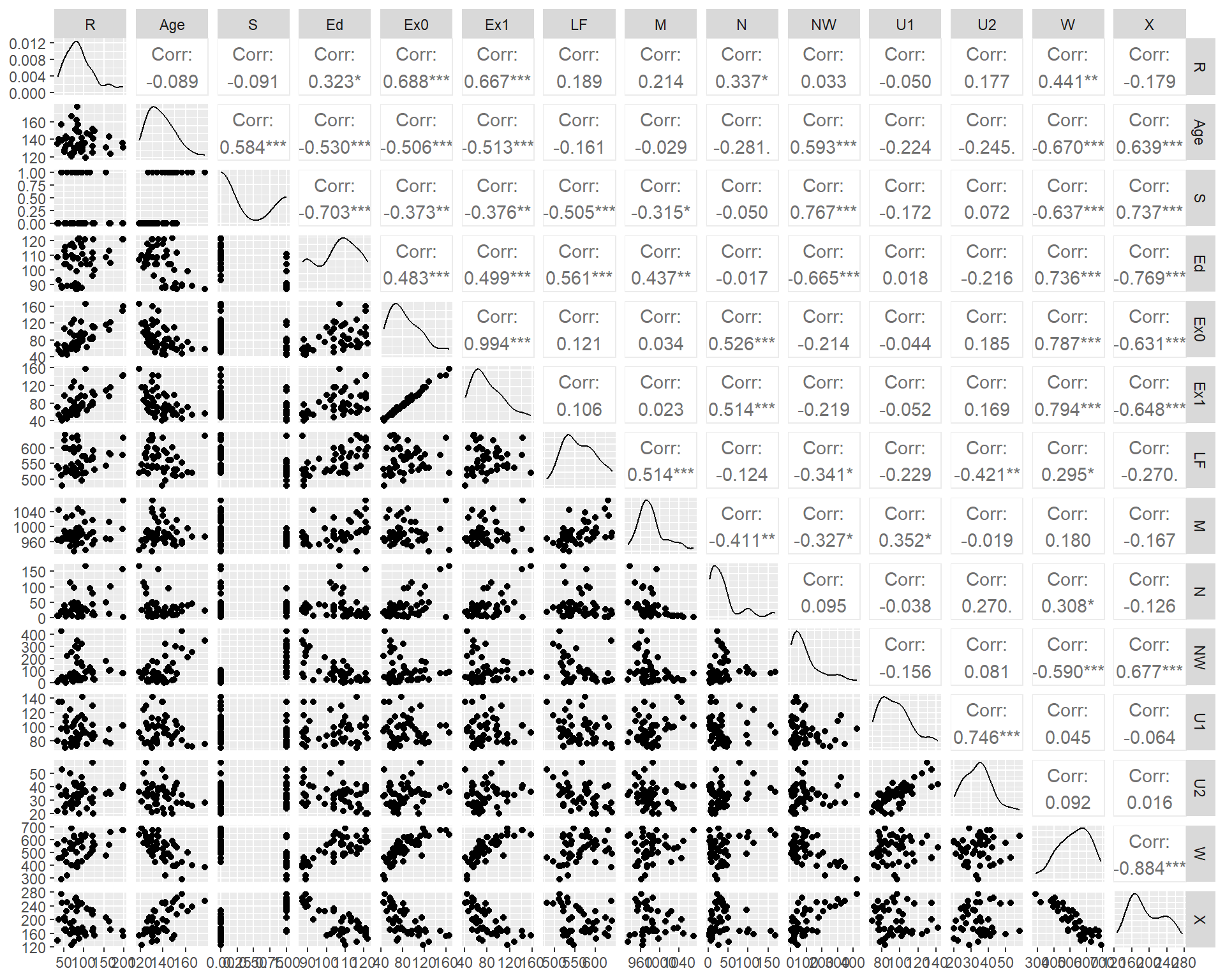
# From the plot above, we can calculate that there have high correlation coefficient between Ex0 and Ex1
cor(usc$Ex0,usc$Ex1)[1] 0.9935865# Show the correlation coefficient directly
ucor <- cor(usc)
ucor R Age S Ed Ex0 Ex1
R 1.00000000 -0.08947240 -0.09063696 0.32283487 0.68760446 0.66671414
Age -0.08947240 1.00000000 0.58435534 -0.53023964 -0.50573690 -0.51317336
S -0.09063696 0.58435534 1.00000000 -0.70274132 -0.37263633 -0.37616753
Ed 0.32283487 -0.53023964 -0.70274132 1.00000000 0.48295213 0.49940958
Ex0 0.68760446 -0.50573690 -0.37263633 0.48295213 1.00000000 0.99358648
Ex1 0.66671414 -0.51317336 -0.37616753 0.49940958 0.99358648 1.00000000
LF 0.18886635 -0.16094882 -0.50546948 0.56117795 0.12149320 0.10634960
M 0.21391426 -0.02867993 -0.31473291 0.43691492 0.03376027 0.02284250
N 0.33747406 -0.28063762 -0.04991832 -0.01722740 0.52628358 0.51378940
NW 0.03259884 0.59319826 0.76710262 -0.66488190 -0.21370878 -0.21876821
U1 -0.05047792 -0.22438060 -0.17241931 0.01810345 -0.04369761 -0.05171199
U2 0.17732065 -0.24484339 0.07169289 -0.21568155 0.18509304 0.16922422
W 0.44131995 -0.67005506 -0.63694543 0.73599704 0.78722528 0.79426205
X -0.17902373 0.63921138 0.73718106 -0.76865789 -0.63050025 -0.64815183
LF M N NW U1 U2
R 0.1888663 0.21391426 0.33747406 0.03259884 -0.05047792 0.17732065
Age -0.1609488 -0.02867993 -0.28063762 0.59319826 -0.22438060 -0.24484339
S -0.5054695 -0.31473291 -0.04991832 0.76710262 -0.17241931 0.07169289
Ed 0.5611780 0.43691492 -0.01722740 -0.66488190 0.01810345 -0.21568155
Ex0 0.1214932 0.03376027 0.52628358 -0.21370878 -0.04369761 0.18509304
Ex1 0.1063496 0.02284250 0.51378940 -0.21876821 -0.05171199 0.16922422
LF 1.0000000 0.51355879 -0.12367222 -0.34121444 -0.22939968 -0.42076249
M 0.5135588 1.00000000 -0.41062750 -0.32730454 0.35189190 -0.01869169
N -0.1236722 -0.41062750 1.00000000 0.09515301 -0.03811995 0.27042159
NW -0.3412144 -0.32730454 0.09515301 1.00000000 -0.15645002 0.08090829
U1 -0.2293997 0.35189190 -0.03811995 -0.15645002 1.00000000 0.74592482
U2 -0.4207625 -0.01869169 0.27042159 0.08090829 0.74592482 1.00000000
W 0.2946323 0.17960864 0.30826271 -0.59010707 0.04485720 0.09207166
X -0.2698865 -0.16708869 -0.12629357 0.67731286 -0.06383218 0.01567818
W X
R 0.44131995 -0.17902373
Age -0.67005506 0.63921138
S -0.63694543 0.73718106
Ed 0.73599704 -0.76865789
Ex0 0.78722528 -0.63050025
Ex1 0.79426205 -0.64815183
LF 0.29463231 -0.26988646
M 0.17960864 -0.16708869
N 0.30826271 -0.12629357
NW -0.59010707 0.67731286
U1 0.04485720 -0.06383218
U2 0.09207166 0.01567818
W 1.00000000 -0.88399728
X -0.88399728 1.00000000# Draw the correlation plot divided by two part (numerical & graphic)
corrplot::corrplot(ucor, order = 'AOE', type = "upper", method = "number")
corrplot::corrplot(ucor, order = "AOE", type = "lower", method = "ell",
diag = FALSE, tl.pos = "n", cl.pos = "n", add = TRUE)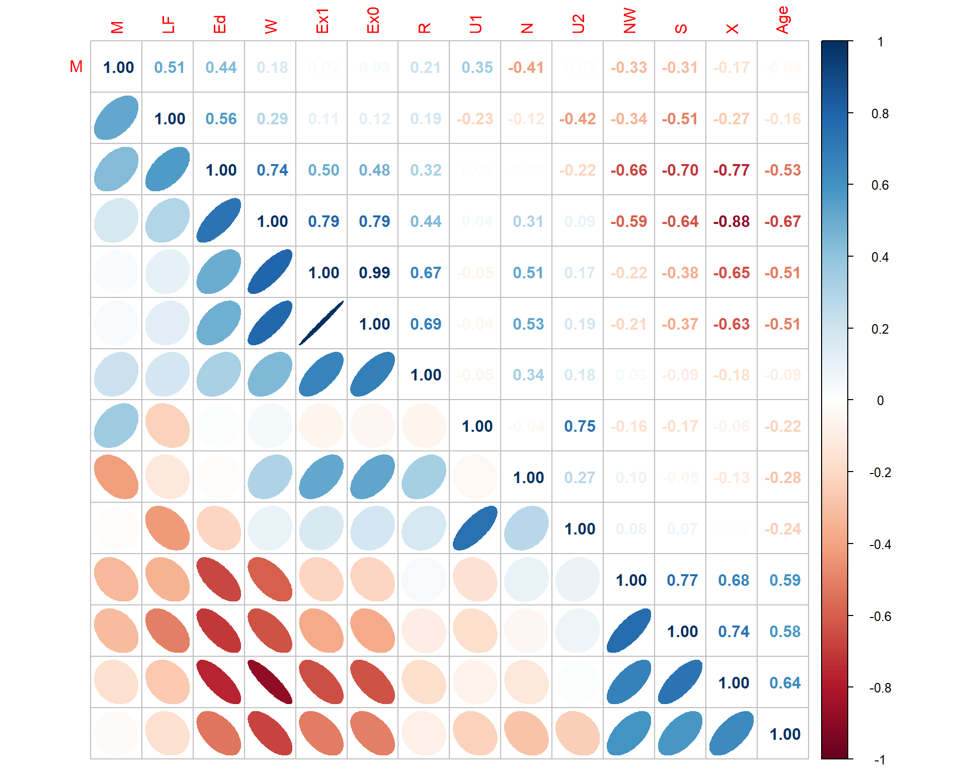
13.3 Fit the model
13.3.1 Analysis
# Do linear regression
crime_rate_lm <- lm(R ~ ., data = usc)
summary(crime_rate_lm)
Call:
lm(formula = R ~ ., data = usc)
Residuals:
Min 1Q Median 3Q Max
-34.884 -11.923 -1.135 13.495 50.560
Coefficients:
Estimate Std. Error t value Pr(>|t|)
(Intercept) -6.918e+02 1.559e+02 -4.438 9.56e-05 ***
Age 1.040e+00 4.227e-01 2.460 0.01931 *
S -8.308e+00 1.491e+01 -0.557 0.58117
Ed 1.802e+00 6.496e-01 2.773 0.00906 **
Ex0 1.608e+00 1.059e+00 1.519 0.13836
Ex1 -6.673e-01 1.149e+00 -0.581 0.56529
LF -4.103e-02 1.535e-01 -0.267 0.79087
M 1.648e-01 2.099e-01 0.785 0.43806
N -4.128e-02 1.295e-01 -0.319 0.75196
NW 7.175e-03 6.387e-02 0.112 0.91124
U1 -6.017e-01 4.372e-01 -1.376 0.17798
U2 1.792e+00 8.561e-01 2.093 0.04407 *
W 1.374e-01 1.058e-01 1.298 0.20332
X 7.929e-01 2.351e-01 3.373 0.00191 **
---
Signif. codes: 0 '***' 0.001 '**' 0.01 '*' 0.05 '.' 0.1 ' ' 1
Residual standard error: 21.94 on 33 degrees of freedom
Multiple R-squared: 0.7692, Adjusted R-squared: 0.6783
F-statistic: 8.462 on 13 and 33 DF, p-value: 3.686e-07# Computes confidence intervals for each parameters in this linear regression model
confint(crime_rate_lm) 2.5 % 97.5 %
(Intercept) -1.008994e+03 -374.6812339
Age 1.798032e-01 1.8998161
S -3.864617e+01 22.0295401
Ed 4.798774e-01 3.1233247
Ex0 -5.460558e-01 3.7616925
Ex1 -3.004455e+00 1.6699389
LF -3.532821e-01 0.2712200
M -2.623148e-01 0.5919047
N -3.047793e-01 0.2222255
NW -1.227641e-01 0.1371135
U1 -1.491073e+00 0.2877222
U2 5.049109e-02 3.5340347
W -7.795484e-02 0.3526718
X 3.146483e-01 1.2712173# Compute analysis of variance tables for this linear regression model
anova(crime_rate_lm)Analysis of Variance Table
Response: R
Df Sum Sq Mean Sq F value Pr(>F)
Age 1 550.8 550.8 1.1448 0.2924072
S 1 153.7 153.7 0.3194 0.5757727
Ed 1 9056.7 9056.7 18.8221 0.0001275 ***
Ex0 1 30760.3 30760.3 63.9278 3.182e-09 ***
Ex1 1 1530.2 1530.2 3.1802 0.0837349 .
LF 1 611.3 611.3 1.2705 0.2677989
M 1 1110.0 1110.0 2.3069 0.1383280
N 1 426.5 426.5 0.8864 0.3533080
NW 1 142.0 142.0 0.2951 0.5906485
U1 1 70.7 70.7 0.1468 0.7040339
U2 1 2696.6 2696.6 5.6043 0.0239336 *
W 1 347.5 347.5 0.7221 0.4015652
X 1 5474.2 5474.2 11.3768 0.0019126 **
Residuals 33 15878.7 481.2
---
Signif. codes: 0 '***' 0.001 '**' 0.01 '*' 0.05 '.' 0.1 ' ' 113.3.2 Conclusion
- The intercept terms, Age, ED, U2, and X are significant variables to explain the crime rate. The 95% confidence intervals also confirm it.
- The model is significant: \(p < 0.05\), adjusted \(R^2 = 0.6783\).
13.3.3 The difference between \(R^2\) and Adj-\(R^2\)
get_R2 <- function(x, method){
round(summary(lm(usc$R ~ as.matrix(usc[, 2:x])))[[method]], 3)
}
dtf_R2 <- data.frame(n = 1:13,
R2 = sapply(2:14, get_R2, method = 'r.squared'),
AdjR2 = sapply(2:14, get_R2, method = 'adj.r.squared'))
library(ggplot2)
library(tidyr)
dtf_R2 |>
pivot_longer(-n) |>
ggplot() +
geom_point(aes(n, value, col = name)) +
geom_line(aes(n, value, col = name))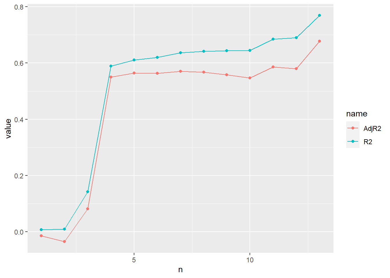
13.4 Evaluate & improve the model
13.4.1 Issue
Multicollinearity:
- multi-: multiple columns
- col-: relationship
- linearity: linear
Problems:
- Imprecise estimates of \(\beta\)
- The t-tests may fail to reveal significant factors
- Missing importance of predictors
# Single linear regression
data(Euphorbiaceae, package = 'gpk')
dtf <- data.frame(x1 = Euphorbiaceae$GBH,
y = Euphorbiaceae$Height)
plot(dtf)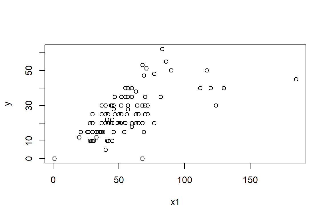
lm(y ~ x1, data = dtf) |> summary()
Call:
lm(formula = y ~ x1, data = dtf)
Residuals:
Min 1Q Median 3Q Max
-29.369 -5.543 -1.566 5.707 28.086
Coefficients:
Estimate Std. Error t value Pr(>|t|)
(Intercept) 8.76295 2.15471 4.067 9.29e-05 ***
x1 0.30303 0.03612 8.390 2.56e-13 ***
---
Signif. codes: 0 '***' 0.001 '**' 0.01 '*' 0.05 '.' 0.1 ' ' 1
Residual standard error: 9.417 on 104 degrees of freedom
Multiple R-squared: 0.4037, Adjusted R-squared: 0.3979
F-statistic: 70.4 on 1 and 104 DF, p-value: 2.564e-13# Multiply linear regression
dtf$x2 <- jitter(dtf$x) # Add some random error to data
pairs(dtf)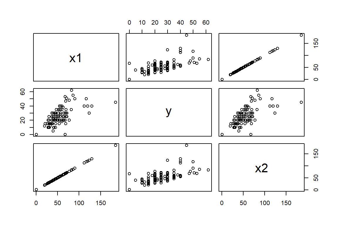
lm(y ~ x1 + x2, data = dtf) |> summary()
Call:
lm(formula = y ~ x1 + x2, data = dtf)
Residuals:
Min 1Q Median 3Q Max
-29.417 -5.501 -1.563 5.707 28.061
Coefficients:
Estimate Std. Error t value Pr(>|t|)
(Intercept) 8.7600 2.1659 4.045 0.000101 ***
x1 0.7077 7.9843 0.089 0.929547
x2 -0.4045 7.9822 -0.051 0.959679
---
Signif. codes: 0 '***' 0.001 '**' 0.01 '*' 0.05 '.' 0.1 ' ' 1
Residual standard error: 9.463 on 103 degrees of freedom
Multiple R-squared: 0.4037, Adjusted R-squared: 0.3921
F-statistic: 34.86 on 2 and 103 DF, p-value: 2.736e-1213.4.2 Variance inflation factor (VIF)
\[\mathrm{VIF}_j = \frac{1}{1-R_j^2}\]
- \(\mathrm{VIF}_j\): \(VIF\) for the \(j\)-th variable
- \(R^2_j\): \(R^2\) from the regression of the \(j\)-th explanatory variable on the remaining explanatory variables.
Remove the R from usc dataset:
uscrimewor <- usc[, -1]
names(uscrimewor) [1] "Age" "S" "Ed" "Ex0" "Ex1" "LF" "M" "N" "NW" "U1" "U2" "W"
[13] "X" Calculate the \(VIF\):
# Compute the VIF for Ex0
usc_lm_Ex0 <- summary(lm(Ex0 ~ ., data = uscrimewor))
1 / (1 - usc_lm_Ex0$r.squared)[1] 94.63312# Compute all of the VIF
faraway::vif(uscrimewor) Age S Ed Ex0 Ex1 LF M N
2.698021 4.876751 5.049442 94.633118 98.637233 3.677557 3.658444 2.324326
NW U1 U2 W X
4.123274 5.938264 4.997617 9.968958 8.409449 Filter: \(VIF > 10\) (\(R^2 > 0.9\))
Drop the variable with highest \(VIF\) and then update the model until all \(VIF \leq 10\):
uscrimewor2 <- uscrimewor[, c('Age','S','Ed','Ex0','LF','M','N','NW','U1','U2','W','X')]
faraway::vif(uscrimewor2) Age S Ed Ex0 LF M N NW
2.670798 4.864533 4.822240 5.109739 3.414298 3.657629 2.321929 3.963407
U1 U2 W X
5.912063 4.982983 9.955587 8.354136 crime_rate_lm2 <- lm(R ~ Age + S + Ed + Ex0 + LF + M + N + NW + U1 + U2 + W + X, usc)
summary(crime_rate_lm2)
Call:
lm(formula = R ~ Age + S + Ed + Ex0 + LF + M + N + NW + U1 +
U2 + W + X, data = usc)
Residuals:
Min 1Q Median 3Q Max
-38.76 -13.59 1.09 13.25 48.93
Coefficients:
Estimate Std. Error t value Pr(>|t|)
(Intercept) -7.041e+02 1.529e+02 -4.604 5.58e-05 ***
Age 1.064e+00 4.165e-01 2.556 0.015226 *
S -7.875e+00 1.475e+01 -0.534 0.596823
Ed 1.722e+00 6.286e-01 2.739 0.009752 **
Ex0 1.010e+00 2.436e-01 4.145 0.000213 ***
LF -1.718e-02 1.464e-01 -0.117 0.907297
M 1.630e-01 2.079e-01 0.784 0.438418
N -3.886e-02 1.282e-01 -0.303 0.763604
NW -1.299e-04 6.200e-02 -0.002 0.998340
U1 -5.848e-01 4.319e-01 -1.354 0.184674
U2 1.819e+00 8.465e-01 2.149 0.038833 *
W 1.351e-01 1.047e-01 1.290 0.205711
X 8.040e-01 2.320e-01 3.465 0.001453 **
---
Signif. codes: 0 '***' 0.001 '**' 0.01 '*' 0.05 '.' 0.1 ' ' 1
Residual standard error: 21.72 on 34 degrees of freedom
Multiple R-squared: 0.7669, Adjusted R-squared: 0.6846
F-statistic: 9.32 on 12 and 34 DF, p-value: 1.351e-07Conclusion: The 12 explanatory variables account for 76.7% of the variability in the crime rates of the 47 states.
13.4.3 Eigen System Analysis
uscrimewor <- as.matrix(uscrimewor)
usc_stan <- scale(uscrimewor)
x1x_stan <- t(usc_stan) %*% usc_stan
usc_eigen <- eigen(x1x_stan)
usc_kappa <- max(usc_eigen$values) / min(usc_eigen$values) # Condition number k- \(k\) < 100: no multicollinearity
- 100 < \(k\) < 1000: moderate multicollinearity
- \(k\) > 1000: severe multicollinearity
usec_index <- max(usc_eigen$values) / usc_eigen$values # Condition indices
usc_eigen$vectors[, usec_index > 1000] [1] -0.010618030 -0.005195201 0.032819351 0.698089398 -0.713641697
[6] -0.033483032 -0.003217082 -0.008582334 0.022697876 -0.004346733
[11] -0.013567474 -0.003024453 -0.015409343We still don’t know which one should be remove, so we’d better use Variance inflation factor (VIF).
13.5 Simply the model
13.5.1 Backward selection
- Start with all the predictors in the model.
- Remove the predictor with highest p-value greater than \(\alpha\) (= 0.05 usually).
- Refit the model and go to 2.
- Stop when all p-values are less than \(\alpha\).
# This function is used to calculate the coefficients of the linear regression model and sort them from largest to smallest by P-value
get_p <- function(model){
smry2 <- data.frame(summary(model)$coefficients)
smry2[order(-smry2$Pr...t..), ]
}
get_p(crime_rate_lm2) Estimate Std..Error t.value Pr...t..
NW -1.299152e-04 0.06200366 -0.002095283 9.983405e-01
LF -1.717960e-02 0.14643342 -0.117320197 9.072966e-01
N -3.886138e-02 0.12818167 -0.303174262 7.636044e-01
S -7.874779e+00 14.74705947 -0.533989803 5.968230e-01
M 1.629746e-01 0.20785304 0.784085841 4.384185e-01
W 1.351072e-01 0.10472364 1.290130466 2.057112e-01
U1 -5.848089e-01 0.43191770 -1.353982319 1.846739e-01
U2 1.819172e+00 0.84648600 2.149086500 3.883343e-02
Age 1.064473e+00 0.41645193 2.556051830 1.522626e-02
Ed 1.721558e+00 0.62864970 2.738501354 9.752489e-03
X 8.040071e-01 0.23201637 3.465303351 1.452904e-03
Ex0 1.009730e+00 0.24359222 4.145163752 2.131854e-04
(Intercept) -7.040822e+02 152.94347802 -4.603545173 5.576618e-05# Update-1
crime_rate_lm3 <- update(crime_rate_lm2, . ~ . - NW)
get_p(crime_rate_lm3) Estimate Std..Error t.value Pr...t..
LF -0.01726849 0.1381358 -0.1250110 9.012301e-01
N -0.03886188 0.1263370 -0.3076048 7.602061e-01
S -7.88953914 12.7694182 -0.6178464 5.406763e-01
M 0.16308486 0.1981909 0.8228675 4.161547e-01
W 0.13515532 0.1007004 1.3421533 1.881884e-01
U1 -0.58495622 0.4200266 -1.3926648 1.725057e-01
U2 1.81920587 0.8341503 2.1809089 3.599816e-02
Age 1.06419549 0.3891918 2.7343726 9.740218e-03
Ed 1.72173268 0.6141343 2.8035115 8.189455e-03
X 0.80399165 0.2285624 3.5176026 1.227429e-03
Ex0 1.00951551 0.2179312 4.6322680 4.846288e-05
(Intercept) -704.12001486 149.6901234 -4.7038509 3.911594e-05# Update-2
crime_rate_lm4 <- update(crime_rate_lm3, . ~ . - LF)
get_p(crime_rate_lm4) Estimate Std..Error t.value Pr...t..
N -0.04145888 0.1229018 -0.3373334 7.378245e-01
S -7.18567759 11.3033138 -0.6357142 5.289835e-01
M 0.15058853 0.1687793 0.8922216 3.781994e-01
W 0.13416908 0.0990088 1.3551227 1.838211e-01
U1 -0.56348963 0.3780445 -1.4905379 1.447935e-01
U2 1.81276664 0.8210969 2.2077377 3.372029e-02
Age 1.06639529 0.3834415 2.7811163 8.565270e-03
Ed 1.70183790 0.5849903 2.9091728 6.175924e-03
X 0.79674056 0.2180364 3.6541625 8.159010e-04
Ex0 1.01443740 0.2113944 4.7987905 2.774137e-05
(Intercept) -700.19856796 144.3514585 -4.8506511 2.369307e-05# Update-3
crime_rate_lm5 <- update(crime_rate_lm4,.~.-N)
get_p(crime_rate_lm5) Estimate Std..Error t.value Pr...t..
S -6.5057045 10.98812498 -0.5920668 5.574067e-01
M 0.1772842 0.14728022 1.2037201 2.363427e-01
W 0.1282847 0.09628581 1.3323326 1.908991e-01
U1 -0.5752009 0.37191143 -1.5466073 1.304695e-01
U2 1.8090238 0.81113002 2.2302513 3.187983e-02
Age 1.0685350 0.37876979 2.8210671 7.651917e-03
Ed 1.7019848 0.57794198 2.9449059 5.556896e-03
X 0.7710981 0.20189436 3.8193147 4.943947e-04
Ex0 0.9833297 0.18792831 5.2324725 6.864110e-06
(Intercept) -716.5469741 134.33461432 -5.3340457 5.005846e-06# Update-4
crime_rate_lm6 <- update(crime_rate_lm5,.~.-S)
get_p(crime_rate_lm6) Estimate Std..Error t.value Pr...t..
M 0.1848948 0.14545901 1.271113 2.114146e-01
W 0.1271449 0.09544037 1.332192 1.907319e-01
U1 -0.5295794 0.36071897 -1.468122 1.503006e-01
U2 1.7070199 0.78581970 2.172279 3.614090e-02
Age 1.0083194 0.36172869 2.787502 8.248097e-03
Ed 1.7416360 0.56912198 3.060216 4.044243e-03
X 0.7320980 0.18920844 3.869267 4.153598e-04
Ex0 0.9785376 0.18614257 5.256926 5.935205e-06
(Intercept) -714.4047282 133.13339398 -5.366082 4.210448e-06# Update-5
crime_rate_lm7 <- update(crime_rate_lm6,.~.-M)
get_p(crime_rate_lm7) Estimate Std..Error t.value Pr...t..
U1 -0.3091858 0.3188025 -0.969835 3.381053e-01
W 0.1454765 0.0950863 1.529942 1.341027e-01
U2 1.4415600 0.7635174 1.888051 6.647498e-02
Age 1.1317545 0.3511903 3.222624 2.566455e-03
Ed 2.0273937 0.5269502 3.847410 4.309248e-04
X 0.7960871 0.1838228 4.330732 1.006325e-04
Ex0 0.9862878 0.1875055 5.260046 5.496412e-06
(Intercept) -614.6654324 108.3983291 -5.670433 1.485771e-06# Update-6
crime_rate_lm8 <- update(crime_rate_lm7,.~.-U1)
get_p(crime_rate_lm8) Estimate Std..Error t.value Pr...t..
W 0.1595649 0.0939003 1.699302 9.702803e-02
U2 0.8281694 0.4273992 1.937695 5.974283e-02
Age 1.1251803 0.3508640 3.206884 2.640080e-03
Ed 1.8178631 0.4802674 3.785106 5.048962e-04
X 0.8235714 0.1814902 4.537828 5.095878e-05
(Intercept) -618.5028439 108.2456006 -5.713884 1.193042e-06
Ex0 1.0506875 0.1752237 5.996264 4.783972e-07# Update-7
crime_rate_lm9 <- update(crime_rate_lm8,.~.-W)
get_p(crime_rate_lm9) Estimate Std..Error t.value Pr...t..
U2 0.9136081 0.4340919 2.104642 4.149584e-02
Age 1.0198219 0.3532027 2.887356 6.175068e-03
Ed 2.0307726 0.4741890 4.282623 1.086147e-04
X 0.6349257 0.1468460 4.323752 9.559356e-05
(Intercept) -524.3743270 95.1155692 -5.513023 2.126586e-06
Ex0 1.2331222 0.1416347 8.706359 7.259666e-11# Final summary
summary(crime_rate_lm9)
Call:
lm(formula = R ~ Age + Ed + Ex0 + U2 + X, data = usc)
Residuals:
Min 1Q Median 3Q Max
-45.344 -9.859 -1.807 10.603 62.964
Coefficients:
Estimate Std. Error t value Pr(>|t|)
(Intercept) -524.3743 95.1156 -5.513 2.13e-06 ***
Age 1.0198 0.3532 2.887 0.006175 **
Ed 2.0308 0.4742 4.283 0.000109 ***
Ex0 1.2331 0.1416 8.706 7.26e-11 ***
U2 0.9136 0.4341 2.105 0.041496 *
X 0.6349 0.1468 4.324 9.56e-05 ***
---
Signif. codes: 0 '***' 0.001 '**' 0.01 '*' 0.05 '.' 0.1 ' ' 1
Residual standard error: 21.3 on 41 degrees of freedom
Multiple R-squared: 0.7296, Adjusted R-squared: 0.6967
F-statistic: 22.13 on 5 and 41 DF, p-value: 1.105e-1013.5.2 Forward selection
- Start with no variables in the model.
- For all predictors not in the model, check their p-value if they are added to the model. Choose the one with lowest p-value less than alpha critical.
- Continue until no new predictors can be added.
13.5.3 AIC selection
Akaike Information Criteria (AIC) principle: big -> bad
crime_rate_aic <- step(crime_rate_lm, direction = "both")Start: AIC=301.66
R ~ Age + S + Ed + Ex0 + Ex1 + LF + M + N + NW + U1 + U2 + W +
X
Df Sum of Sq RSS AIC
- NW 1 6.1 15885 299.68
- LF 1 34.4 15913 299.76
- N 1 48.9 15928 299.81
- S 1 149.4 16028 300.10
- Ex1 1 162.3 16041 300.14
- M 1 296.5 16175 300.53
<none> 15879 301.66
- W 1 810.6 16689 302.00
- U1 1 911.5 16790 302.29
- Ex0 1 1109.8 16989 302.84
- U2 1 2108.8 17988 305.52
- Age 1 2911.6 18790 307.57
- Ed 1 3700.5 19579 309.51
- X 1 5474.2 21353 313.58
Step: AIC=299.68
R ~ Age + S + Ed + Ex0 + Ex1 + LF + M + N + U1 + U2 + W + X
Df Sum of Sq RSS AIC
- LF 1 28.7 15913 297.76
- N 1 48.6 15933 297.82
- Ex1 1 156.3 16041 298.14
- S 1 158.0 16043 298.14
- M 1 294.1 16179 298.54
<none> 15885 299.68
- W 1 820.2 16705 300.05
- U1 1 913.1 16798 300.31
- Ex0 1 1104.3 16989 300.84
+ NW 1 6.1 15879 301.66
- U2 1 2107.1 17992 303.53
- Age 1 3365.8 19251 306.71
- Ed 1 3757.1 19642 307.66
- X 1 5503.6 21388 311.66
Step: AIC=297.76
R ~ Age + S + Ed + Ex0 + Ex1 + M + N + U1 + U2 + W + X
Df Sum of Sq RSS AIC
- N 1 62.2 15976 295.95
- S 1 129.4 16043 296.14
- Ex1 1 134.8 16048 296.16
- M 1 276.8 16190 296.57
<none> 15913 297.76
- W 1 801.9 16715 298.07
- U1 1 941.8 16855 298.47
- Ex0 1 1075.9 16989 298.84
+ LF 1 28.7 15885 299.68
+ NW 1 0.3 15913 299.76
- U2 1 2088.5 18002 301.56
- Age 1 3407.9 19321 304.88
- Ed 1 3895.3 19809 306.06
- X 1 5621.3 21535 309.98
Step: AIC=295.95
R ~ Age + S + Ed + Ex0 + Ex1 + M + U1 + U2 + W + X
Df Sum of Sq RSS AIC
- S 1 104.4 16080 294.25
- Ex1 1 123.3 16099 294.31
- M 1 533.8 16509 295.49
<none> 15976 295.95
- W 1 748.7 16724 296.10
- U1 1 997.7 16973 296.80
- Ex0 1 1021.3 16997 296.86
+ N 1 62.2 15913 297.76
+ LF 1 42.3 15933 297.82
+ NW 1 0.0 15976 297.95
- U2 1 2082.3 18058 299.71
- Age 1 3425.9 19402 303.08
- Ed 1 3887.6 19863 304.19
- X 1 5896.9 21873 308.71
Step: AIC=294.25
R ~ Age + Ed + Ex0 + Ex1 + M + U1 + U2 + W + X
Df Sum of Sq RSS AIC
- Ex1 1 171.5 16252 292.75
- M 1 563.4 16643 293.87
<none> 16080 294.25
- W 1 734.7 16815 294.35
- U1 1 906.0 16986 294.83
- Ex0 1 1162.0 17242 295.53
+ S 1 104.4 15976 295.95
+ N 1 37.2 16043 296.14
+ NW 1 14.2 16066 296.21
+ LF 1 1.9 16078 296.25
- U2 1 1978.0 18058 297.71
- Age 1 3354.5 19434 301.16
- Ed 1 4139.1 20219 303.02
- X 1 6094.8 22175 307.36
Step: AIC=292.75
R ~ Age + Ed + Ex0 + M + U1 + U2 + W + X
Df Sum of Sq RSS AIC
- M 1 691.0 16943 292.71
<none> 16252 292.75
- W 1 759.0 17011 292.90
- U1 1 921.8 17173 293.35
+ Ex1 1 171.5 16080 294.25
+ S 1 152.5 16099 294.31
+ NW 1 36.0 16215 294.65
+ N 1 23.1 16228 294.69
+ LF 1 5.5 16246 294.74
- U2 1 2018.1 18270 296.25
- Age 1 3323.1 19575 299.50
- Ed 1 4005.1 20257 301.11
- X 1 6402.7 22654 306.36
- Ex0 1 11818.8 28070 316.44
Step: AIC=292.71
R ~ Age + Ed + Ex0 + U1 + U2 + W + X
Df Sum of Sq RSS AIC
- U1 1 408.6 17351 291.83
<none> 16943 292.71
+ M 1 691.0 16252 292.75
- W 1 1016.9 17959 293.45
+ Ex1 1 299.0 16643 293.87
+ N 1 262.5 16680 293.98
+ LF 1 213.3 16729 294.11
+ S 1 213.1 16729 294.11
+ NW 1 114.2 16828 294.39
- U2 1 1548.6 18491 294.82
- Age 1 4511.6 21454 301.81
- Ed 1 6430.6 23373 305.83
- X 1 8147.7 25090 309.16
- Ex0 1 12019.6 28962 315.91
Step: AIC=291.83
R ~ Age + Ed + Ex0 + U2 + W + X
Df Sum of Sq RSS AIC
<none> 17351 291.83
+ U1 1 408.6 16942 292.71
- W 1 1252.6 18604 293.11
+ Ex1 1 251.2 17100 293.14
+ LF 1 230.7 17120 293.20
+ N 1 189.6 17162 293.31
+ M 1 177.8 17173 293.35
+ S 1 71.0 17280 293.64
+ NW 1 59.2 17292 293.67
- U2 1 1628.7 18980 294.05
- Age 1 4461.0 21812 300.58
- Ed 1 6214.7 23566 304.22
- X 1 8932.3 26283 309.35
- Ex0 1 15596.5 32948 319.97summary(crime_rate_aic)
Call:
lm(formula = R ~ Age + Ed + Ex0 + U2 + W + X, data = usc)
Residuals:
Min 1Q Median 3Q Max
-38.306 -10.209 -1.313 9.919 54.544
Coefficients:
Estimate Std. Error t value Pr(>|t|)
(Intercept) -618.5028 108.2456 -5.714 1.19e-06 ***
Age 1.1252 0.3509 3.207 0.002640 **
Ed 1.8179 0.4803 3.785 0.000505 ***
Ex0 1.0507 0.1752 5.996 4.78e-07 ***
U2 0.8282 0.4274 1.938 0.059743 .
W 0.1596 0.0939 1.699 0.097028 .
X 0.8236 0.1815 4.538 5.10e-05 ***
---
Signif. codes: 0 '***' 0.001 '**' 0.01 '*' 0.05 '.' 0.1 ' ' 1
Residual standard error: 20.83 on 40 degrees of freedom
Multiple R-squared: 0.7478, Adjusted R-squared: 0.71
F-statistic: 19.77 on 6 and 40 DF, p-value: 1.441e-1013.5.4 Result
According to the backward selection:
equatiomatic::extract_eq(crime_rate_lm9, use_coefs = TRUE)\[ \operatorname{\widehat{R}} = -524.37 + 1.02(\operatorname{Age}) + 2.03(\operatorname{Ed}) + 1.23(\operatorname{Ex0}) + 0.91(\operatorname{U2}) + 0.63(\operatorname{X}) \]
stargazer::stargazer(crime_rate_lm9, type = 'text')
===============================================
Dependent variable:
---------------------------
R
-----------------------------------------------
Age 1.020***
(0.353)
Ed 2.031***
(0.474)
Ex0 1.233***
(0.142)
U2 0.914**
(0.434)
X 0.635***
(0.147)
Constant -524.374***
(95.116)
-----------------------------------------------
Observations 47
R2 0.730
Adjusted R2 0.697
Residual Std. Error 21.301 (df = 41)
F Statistic 22.129*** (df = 5; 41)
===============================================
Note: *p<0.1; **p<0.05; ***p<0.01The model shows that the variables Age, Ed, Ex0, U2, and X explain 73% of the variability in the crime rates.
According to the AIC selection:
equatiomatic::extract_eq(crime_rate_aic, use_coefs = TRUE)\[ \operatorname{\widehat{R}} = -618.5 + 1.13(\operatorname{Age}) + 1.82(\operatorname{Ed}) + 1.05(\operatorname{Ex0}) + 0.83(\operatorname{U2}) + 0.16(\operatorname{W}) + 0.82(\operatorname{X}) \]
stargazer::stargazer(crime_rate_aic, type = 'text')
===============================================
Dependent variable:
---------------------------
R
-----------------------------------------------
Age 1.125***
(0.351)
Ed 1.818***
(0.480)
Ex0 1.051***
(0.175)
U2 0.828*
(0.427)
W 0.160*
(0.094)
X 0.824***
(0.181)
Constant -618.503***
(108.246)
-----------------------------------------------
Observations 47
R2 0.748
Adjusted R2 0.710
Residual Std. Error 20.827 (df = 40)
F Statistic 19.771*** (df = 6; 40)
===============================================
Note: *p<0.1; **p<0.05; ***p<0.01The model shows that the variables Age, Ed, Ex0, U2, W, and X explain 75% of the variability in the crime rates.
14 Logistic regression
14.1 Limitation of linear model
Some limitations of linear models:
- Out of the range of possible y
- The residuals-vs-predicted plot indicates two parallel lines, which is very unlikely if a linear model is appropriate.
# Scatter plot + abline
library(ggplot2)
iris2 <- iris[iris$Species %in% c('versicolor', 'setosa'),
c('Species', 'Sepal.Length', 'Petal.Length')]
iris2$SpeciesLevel <- as.integer(iris2$Species) - 1 # 0: setosa. 1:versicolor
ggplot(iris2) +
geom_point(aes(Sepal.Length, SpeciesLevel), alpha = 0.2, size = 6) +
geom_smooth(aes(Sepal.Length, SpeciesLevel), method = 'lm')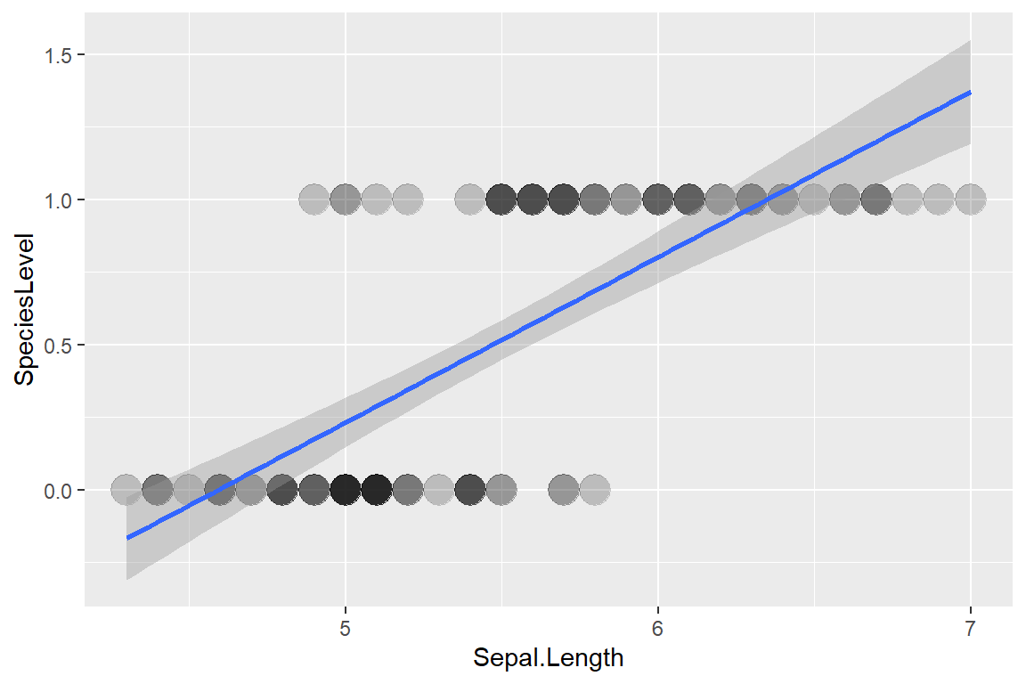
# Check the statistic analysis
lm_iris2 <- lm(SpeciesLevel ~ Sepal.Length, data = iris2)
summary(lm_iris2)
Call:
lm(formula = SpeciesLevel ~ Sepal.Length, data = iris2)
Residuals:
Min 1Q Median 3Q Max
-0.68764 -0.23802 -0.04506 0.25533 0.82566
Coefficients:
Estimate Std. Error t value Pr(>|t|)
(Intercept) -2.62027 0.29859 -8.776 5.47e-14 ***
Sepal.Length 0.57033 0.05421 10.521 < 2e-16 ***
---
Signif. codes: 0 '***' 0.001 '**' 0.01 '*' 0.05 '.' 0.1 ' ' 1
Residual standard error: 0.3461 on 98 degrees of freedom
Multiple R-squared: 0.5304, Adjusted R-squared: 0.5256
F-statistic: 110.7 on 1 and 98 DF, p-value: < 2.2e-16# Multiply residual plots
par(mfrow = c(2, 2))
plot(lm_iris2)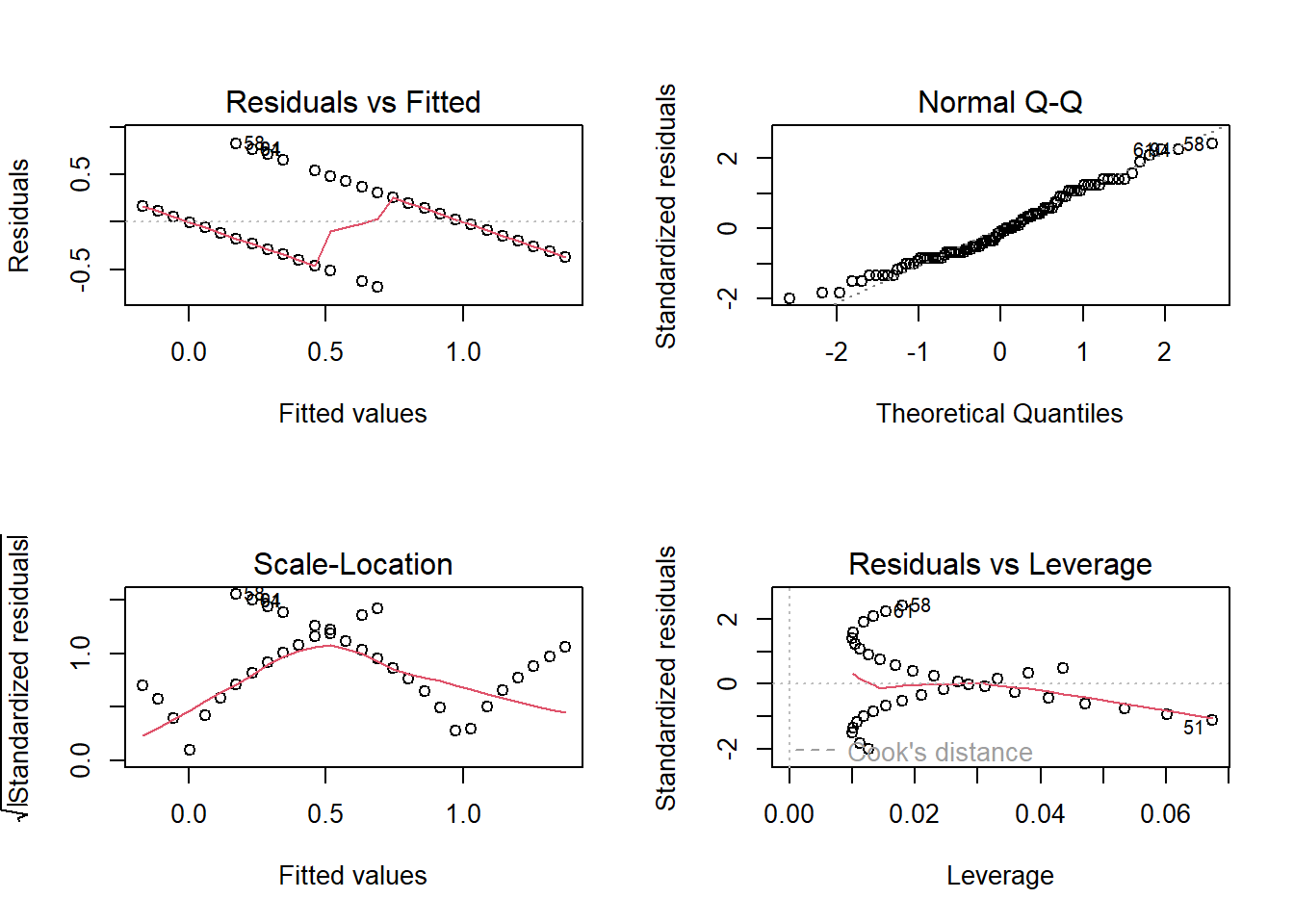
So we can use those code instead of the previous one:
iris2$SepalBin <- round(iris2$Sepal.Length * 4) / 4
iris_tbl <- table(iris2$SepalBin, iris2$SpeciesLevel)
iris_p <- data.frame(cbind(iris_tbl))
iris_p$SepalBin <- as.numeric(row.names(iris_p))
iris_p$p <- iris_p$X1 / (iris_p$X0 + iris_p$X1) # Proportion of versicolor
ggplot(iris_p) + geom_point(aes(SepalBin, p))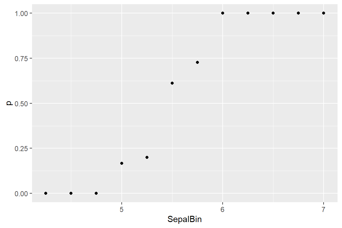
Then we can use the Sigmoid curve: \(\frac{\ 1}{\ 1 +e^{-x}}\) to describe this relationship:
curve(1 / (1 + exp(-x)), xlim = c(-10, 10))
abline(h = 0:1, col = "royalblue4",lty = 2)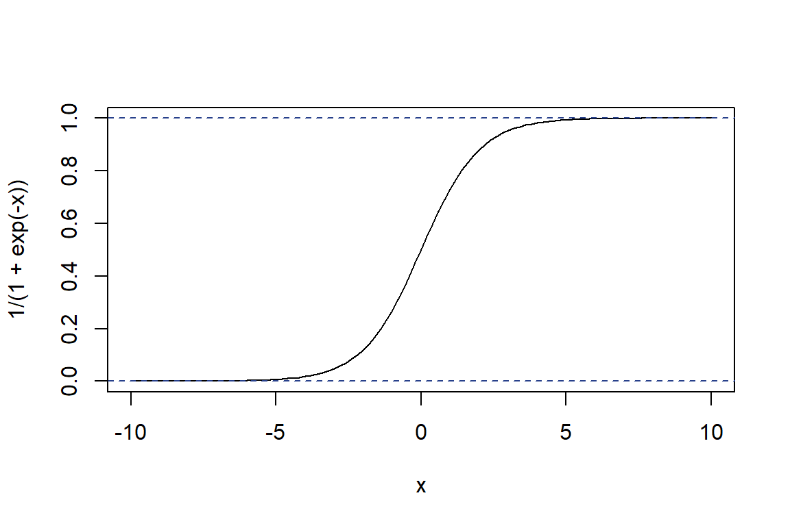
14.2 Binary logistic regression
14.2.1 Concept
(Binary) Logistic regression:
Use a logistic function to model a binary dependent variable (1/0, yes/no, true/false, win/lose, male/female) against one or multiple qualitative variables. \[log \frac{p(X)}{1-p(X)} = \beta_0 + \beta_1 X_1 + \beta_2 X_2 + ... + \beta_pX_p\] Can convert into: \[p(X) = \frac{e^{\beta_0 + \beta_1X_1 + \beta_2X_2 + … + \beta_pX_p}}{\ (1 + e^{\beta_0 + \beta_1X_1 + \beta_2X_2 + … + \beta_pX_p})}\]
- \(X_i\): The \(i\)-th predictor variable
- \(\beta_i\): The coefficient estimate for the \(i\)-th predictor variable
14.2.2 Example
14.2.2.1 Fit the model
Iris data:
# Check the iris2 structure
head(iris2, 3) Species Sepal.Length Petal.Length SpeciesLevel SepalBin
1 setosa 5.1 1.4 0 5.00
2 setosa 4.9 1.4 0 5.00
3 setosa 4.7 1.3 0 4.75# Summarize the statistic analysis on iris2 dataset between SpeciesLevel & Sepal.Length
lg_iris1 <- glm(SpeciesLevel ~ Sepal.Length, data = iris2, family = binomial)
summary(lg_iris1)
Call:
glm(formula = SpeciesLevel ~ Sepal.Length, family = binomial,
data = iris2)
Deviance Residuals:
Min 1Q Median 3Q Max
-2.05501 -0.47395 -0.02829 0.39788 2.32915
Coefficients:
Estimate Std. Error z value Pr(>|z|)
(Intercept) -27.831 5.434 -5.122 3.02e-07 ***
Sepal.Length 5.140 1.007 5.107 3.28e-07 ***
---
Signif. codes: 0 '***' 0.001 '**' 0.01 '*' 0.05 '.' 0.1 ' ' 1
(Dispersion parameter for binomial family taken to be 1)
Null deviance: 138.629 on 99 degrees of freedom
Residual deviance: 64.211 on 98 degrees of freedom
AIC: 68.211
Number of Fisher Scoring iterations: 6# McFadden pseudo-R squared is a statistic used to evaluate the goodness of fit of logistic regression models
# The greater, the more important, when value is 0.2~0.4 then it is very good
pscl::pR2(lg_iris1)["McFadden"]fitting null model for pseudo-r2 McFadden
0.5368136 # Extract the formula from lg_iris1
equatiomatic::extract_eq(lg_iris1, use_coefs = TRUE)\[ \log\left[ \frac { \widehat{P( \operatorname{SpeciesLevel} = \operatorname{1} )} }{ 1 - \widehat{P( \operatorname{SpeciesLevel} = \operatorname{1} )} } \right] = -27.83 + 5.14(\operatorname{Sepal.Length}) \]
# Show the statistic result
stargazer::stargazer(lg_iris1, type = 'text')
=============================================
Dependent variable:
---------------------------
SpeciesLevel
---------------------------------------------
Sepal.Length 5.140***
(1.007)
Constant -27.831***
(5.434)
---------------------------------------------
Observations 100
Log Likelihood -32.106
Akaike Inf. Crit. 68.211
=============================================
Note: *p<0.1; **p<0.05; ***p<0.0114.2.2.2 Assess the model
# Do the statistic analysis on iris2 dataset between SpeciesLevel & Sepal.Length + Petal.Length
lg_iris2 <- glm(SpeciesLevel ~ Sepal.Length + Petal.Length, data = iris2, family = binomial)
# Understand which predictive variables contribute significantly to the predictive power of the model
# The greater, the more important
caret::varImp(lg_iris2) Overall
Sepal.Length 0.0002083317
Petal.Length 0.0006938295# Extract the formula from lg_iris2
equatiomatic::extract_eq(lg_iris2, use_coefs = TRUE)\[ \log\left[ \frac { \widehat{P( \operatorname{SpeciesLevel} = \operatorname{1} )} }{ 1 - \widehat{P( \operatorname{SpeciesLevel} = \operatorname{1} )} } \right] = 65.84 - 37.56(\operatorname{Sepal.Length}) + 49.05(\operatorname{Petal.Length}) \]
# Show the statistic result
stargazer::stargazer(lg_iris2, type = 'text')
=============================================
Dependent variable:
---------------------------
SpeciesLevel
---------------------------------------------
Sepal.Length -37.561
(180,296.200)
Petal.Length 49.046
(70,689.070)
Constant 65.843
(744,553.200)
---------------------------------------------
Observations 100
Log Likelihood -0.000
Akaike Inf. Crit. 6.000
=============================================
Note: *p<0.1; **p<0.05; ***p<0.0114.2.2.3 Visualization
# Fit a liner regression line on it
ggplot(iris2, aes(x=Sepal.Length, y=SpeciesLevel)) +
geom_point() +
geom_smooth(method="glm", method.args = list(family=binomial)) +
labs(x = 'Sepal length (cm)', y = 'Species and p')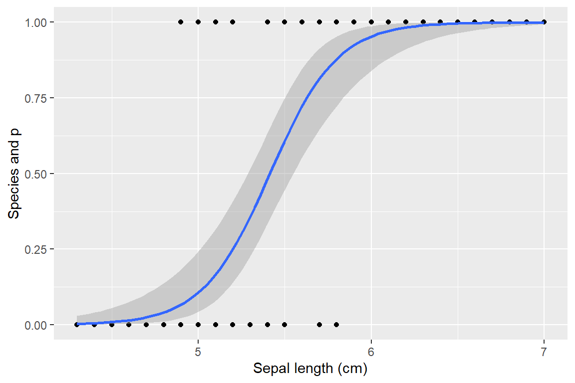
14.3 Multinomial and ordinal logistic regression
14.3.1 Concept
Multinomial logistic regression:
Use a logistic function to model a nominal variable with multiple levels against one or multiple qualitative variables.
Ordinal logistic regression:
Use a logistic function to model a ordinal variable with multiple levels against one or multiple qualitative variables.
14.3.1.1 As a Model for Odds
\[\frac{P(Y{i}=j|X{i})}{P(Y{i}=J|X{i})}=exp[\alpha_{j}+\beta_{j}x_{i}]\]
- \(j\): level of the dependent variable. 1, …, \(J\)
- \(P(Y{i}=j|X{i})\): The probability that individual \(i\) is in level \(j\) given a value of \(x_i\).
- The \(J\)-th* level: the baseline.
14.3.1.2 As a Model of Probabilities
\[{P(Y{i}=j|X{i})}=\frac{exp[\alpha_{j}+\beta_{j}x_{i}]}{\sum_{h=1}^{J}exp[\alpha_{h}+\beta_{h}x_{i}]},\quad where \,\, j = 1,...,J\]
14.3.2 Example
14.3.2.1 Prepare the data
The iris dataset. Can we predict the Species according to the sepal and petal lengths and widths?
- Dependent variable: Species (a categorical variable with 3 levels)
- Independent variables: Sepal and petal lengths and widths (4 numerical variables)?
Separate the dataset into training data (80%) and test data (20%) randomly:
set.seed(123)
train.sub <- sample(nrow(iris), round(0.8 * nrow(iris)))
train.data <- iris[train.sub, ]
test.data <- iris[-train.sub, ] 14.3.2.2 Fit the model
- Only two species displayed: setosa as the baseline level
library(nnet)
model <- multinom(Species ~ ., data = train.data)# weights: 18 (10 variable)
initial value 131.833475
iter 10 value 12.430734
iter 20 value 2.945373
iter 30 value 2.027434
iter 40 value 1.883088
iter 50 value 1.835737
iter 60 value 1.697733
iter 70 value 1.351628
iter 80 value 0.944059
iter 90 value 0.776663
iter 100 value 0.737237
final value 0.737237
stopped after 100 iterationssummary(model)Call:
multinom(formula = Species ~ ., data = train.data)
Coefficients:
(Intercept) Sepal.Length Sepal.Width Petal.Length Petal.Width
versicolor 48.28722 -24.64201 -24.27893 47.2458 3.130761
virginica -83.41388 -58.94158 -60.89885 117.6548 65.130414
Std. Errors:
(Intercept) Sepal.Length Sepal.Width Petal.Length Petal.Width
versicolor 106.5370 35.94035 27.03289 48.92239 32.11012
virginica 105.9997 46.24989 32.56462 41.91175 29.42979
Residual Deviance: 1.474475
AIC: 21.47447 \[O_{ve}=\frac{P(Y_i=versicolor)}{P(Y_i=setosa)} = exp(48.28722 - 24.64201L_s - 24.27893W_s + 47.2458L_p + 3.130761W_p)\] \[O_{vi} = \frac{P(Y_i=virginica)}{P(Y_i=setosa)} = exp(-83.41388 - 58.94158L_s - 60.89885W_s + 117.6548L_p + 65.130414W_p)\]
14.3.2.3 Validate the model
# Prediction
o_ve <- exp(48.28722 - 24.64201 * test.data$Sepal.Length[1] - 24.27893 * test.data$Sepal.Width[1] + 47.2458 * test.data$Petal.Length[1] + 3.130761 * test.data$Petal.Width[1])
o_vi <- exp(-83.41388 - 58.94158 * test.data$Sepal.Length[1] - 60.89885 * test.data$Sepal.Width[1] + 117.6548 * test.data$Petal.Length[1] + 65.130414 * test.data$Petal.Width[1])
p_ve <- o_ve / (o_ve + o_vi + 1)
p_vi <- o_vi / (o_ve + o_vi + 1)
p_se <- 1 - p_ve - p_vi
# Check the recall
test.data$predicted <- predict(model, newdata = test.data)
mean(test.data$predicted == test.data$Species) # rate[1] 0.9666667table(test.data$Species, test.data$predicted) # matrix
setosa versicolor virginica
setosa 10 0 0
versicolor 0 14 1
virginica 0 0 5# Visualize in a diagram which showing the prediction result distribution
predicted.data1 <- data.frame(probability.of.Species = model$fitted.values, Species=train.data$Species)
predicted.data1$n <- 1:nrow(predicted.data1)
library(ggplot2)
ggplot(predicted.data1, aes(n,probability.of.Species.versicolor)) +
geom_point(aes(color=Species)) +
xlab("n") +
ylab("Predicted probability of versicolor")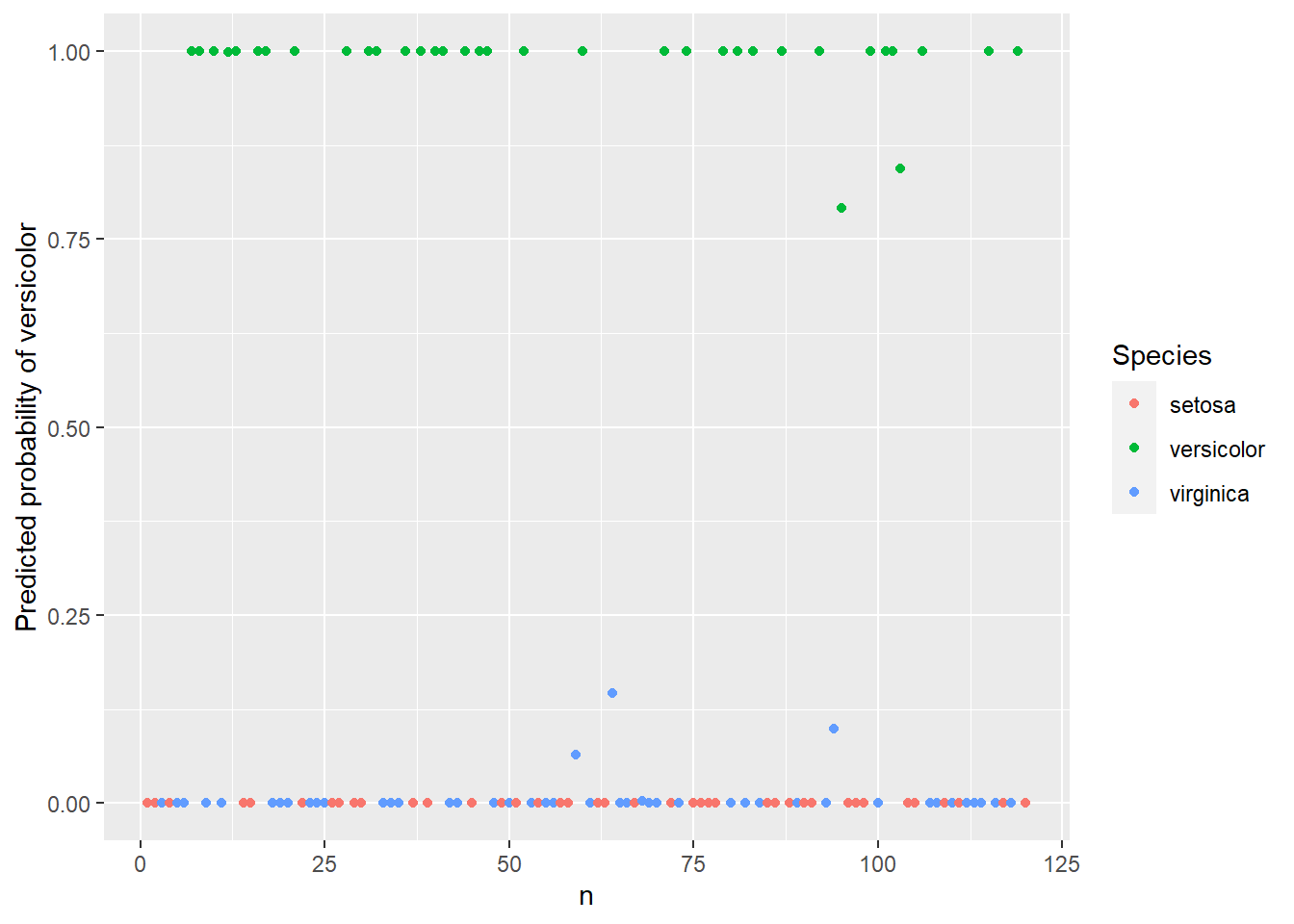
Wald test:
Determine the significance of odds ratios in logistic regression model and calculate confidence interval.
- \(H_0\): \(\beta = 0\) (the Wald statistic is an approximate standard normal distribution) \[z_{score} =\frac{β}{s_e}\]
Z-score & P-value:
z_score <- summary(model)$coefficients/summary(model)$standard.errors
z_score (Intercept) Sepal.Length Sepal.Width Petal.Length Petal.Width
versicolor 0.4532436 -0.6856363 -0.8981256 0.9657296 0.09750075
virginica -0.7869252 -1.2744157 -1.8700922 2.8072031 2.21307796p <- pnorm(abs(z_score), lower.tail = FALSE) * 2
p (Intercept) Sepal.Length Sepal.Width Petal.Length Petal.Width
versicolor 0.6503733 0.4929425 0.36911861 0.334179508 0.92232874
virginica 0.4313256 0.2025161 0.06147101 0.004997373 0.02689227Confidence intervals:
confint(model) # One step, , versicolor
2.5 % 97.5 %
(Intercept) -160.52147 257.09590
Sepal.Length -95.08380 45.79978
Sepal.Width -77.26243 28.70456
Petal.Length -48.64032 143.13193
Petal.Width -59.80392 66.06544
, , virginica
2.5 % 97.5 %
(Intercept) -291.16957 124.341812
Sepal.Length -149.58970 31.706534
Sepal.Width -124.72434 2.926639
Petal.Length 35.50928 199.800337
Petal.Width 7.44909 122.81173814.3.2.4 Simply the model
AIC filter:
# Evaluate and improve the model automatic (In this example we already get the best model)
model2 <- step(model)
summary(model2)
z_score <- summary(model2)$coefficients/summary(model2)$standard.errors
z_score
p <- pnorm(abs(z_score), lower.tail = FALSE) * 2
pVIF filter: VIF > 10 (R2 > 0.9)
# Test
iriswor <- train.data[, 1:4]
faraway::vif(iriswor)Sepal.Length Sepal.Width Petal.Length Petal.Width
6.946158 2.005345 29.045187 14.758382 # Filter
iriswor2 <- iriswor[, c('Sepal.Length', 'Sepal.Width')]
faraway::vif(iriswor2)Sepal.Length Sepal.Width
1.012571 1.012571 # Update
model3 <- multinom(Species ~ Sepal.Length + Sepal.Width, data = train.data)# weights: 12 (6 variable)
initial value 131.833475
iter 10 value 50.835156
iter 20 value 49.035250
iter 30 value 44.711778
iter 40 value 44.640621
iter 50 value 44.625237
iter 60 value 44.602328
iter 70 value 44.573805
iter 80 value 44.553198
iter 90 value 44.535668
iter 100 value 44.527089
final value 44.527089
stopped after 100 iterationssummary(model3)Call:
multinom(formula = Species ~ Sepal.Length + Sepal.Width, data = train.data)
Coefficients:
(Intercept) Sepal.Length Sepal.Width
versicolor -67.69944 26.75297 -24.22665
virginica -79.78359 28.56638 -23.85885
Std. Errors:
(Intercept) Sepal.Length Sepal.Width
versicolor 59.21976 20.84157 18.96879
virginica 59.32647 20.84901 18.97688
Residual Deviance: 89.05418
AIC: 101.0542 z_score <- summary(model3)$coefficients/summary(model3)$standard.errors
z_score (Intercept) Sepal.Length Sepal.Width
versicolor -1.143190 1.283635 -1.277185
virginica -1.344823 1.370155 -1.257259p <- pnorm(abs(z_score), lower.tail = FALSE) * 2
p (Intercept) Sepal.Length Sepal.Width
versicolor 0.2529597 0.1992697 0.2015371
virginica 0.1786824 0.1706384 0.208659814.3.2.5 Result
stargazer::stargazer(model, type = 'text')
==============================================
Dependent variable:
----------------------------
versicolor virginica
(1) (2)
----------------------------------------------
Sepal.Length -24.642 -58.942
(35.940) (46.250)
Sepal.Width -24.279 -60.899*
(27.033) (32.565)
Petal.Length 47.246 117.655***
(48.922) (41.912)
Petal.Width 3.131 65.130**
(32.110) (29.430)
Constant 48.287 -83.414
(106.537) (106.000)
----------------------------------------------
Akaike Inf. Crit. 21.474 21.474
==============================================
Note: *p<0.1; **p<0.05; ***p<0.0115 Poisson regression
15.1 Concept
15.1.1 Definition
Poisson distribution:
A discrete probability distribution. The probability of occurrence of an event in a fixed spatial or temporal scales.
Derived from the binomial distribution for an infinite number of binomial distributions and an infinitesimal probability of each occurrence.
PDF for Poisson distribution (\(\lambda\) instead of \(\mu\) in binomial distribution): \[P\left( X=k \right)=\frac{\lambda^{k}}{k!}e^{-\lambda}\]
- \(P\left( X=k \right)\) represents the probability of a random event occurring \(k\) times per unit time
- \(k=0,1,2,...\)
- \(\lambda >0\) (the expected value of x)
# Compare Poisson distribution with Normal distribution
for (l in 1:5) {
curve(dpois(x, l),
from = 0, to = 10, n = 11,
add = l > 1, col = l,
ylab = 'Density', lwd = 3)
}
legend('topright', legend = 1:5, title = bquote(lambda),
lty = 1, col = 1:5, lwd = 3)
for (l in 1:5) {
curve(dnorm(x, mean = l, sd = sqrt(l)),
from = 0, to = 10, n = 110,
col = l, lty = 2,
add = TRUE)
}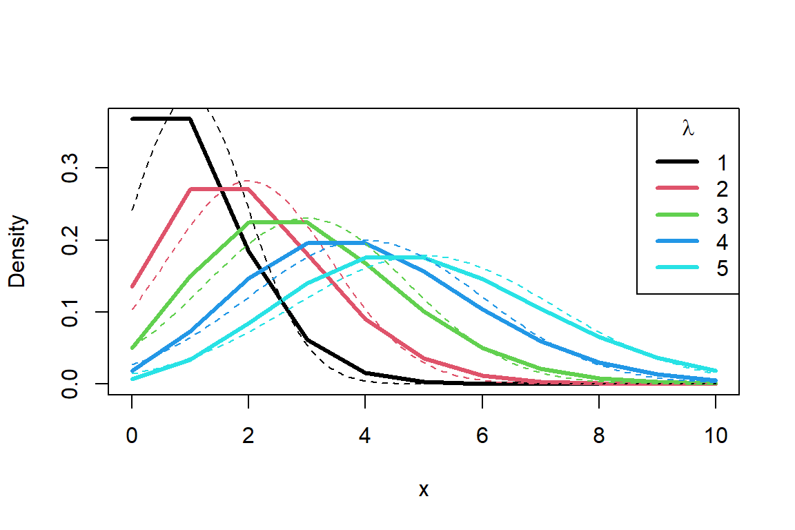
15.1.2 Features of Poisson distribution
- \(\mu=\sigma^2=\lambda\)
- If \(Y_1\) ~Poisson (\(\lambda_1\)), \(Y_2\)~Poisson(\(\lambda_2\)), then \(Y=Y1+Y2\)~Poisson(\(\lambda=\lambda_1+\lambda_2\))
- With the increase of \(\lambda\), the center of the distribution moves to the right, and the Poisson distribution approaches the normal distribution.
15.1.3 Assumptions
- The occurrence of an event is completely random.
- The occurrence of an event is independent.
- The probability \(p\) of the occurrence of an event remains unchanged.
- The probability \(p\) of the event is low and the sample size is large.
15.1.4 Model
\[log(Y)=a + b_1x_1 + b_2x_2 + b_nx_n.....\]
- \(Y\): response variable
- \(a\) and \(b\): numerical coefficients
- \(x\): predictive variable
15.2 Workflow
15.2.1 Fit model
Count of the plant species ~ the geographic variables
library(faraway)
data(gala)
fit.gala <-
glm(
Species ~ Endemics + Area + Elevation + Nearest + Scruz + Adjacent,
data = gala,
family = poisson()
)
summary(fit.gala)
Call:
glm(formula = Species ~ Endemics + Area + Elevation + Nearest +
Scruz + Adjacent, family = poisson(), data = gala)
Deviance Residuals:
Min 1Q Median 3Q Max
-4.9919 -2.9305 -0.4296 1.3254 7.4735
Coefficients:
Estimate Std. Error z value Pr(>|z|)
(Intercept) 2.828e+00 5.958e-02 47.471 < 2e-16 ***
Endemics 3.388e-02 1.741e-03 19.459 < 2e-16 ***
Area -1.067e-04 3.741e-05 -2.853 0.00433 **
Elevation 2.638e-04 1.934e-04 1.364 0.17264
Nearest 1.048e-02 1.611e-03 6.502 7.91e-11 ***
Scruz -6.835e-04 5.802e-04 -1.178 0.23877
Adjacent 4.539e-05 4.800e-05 0.946 0.34437
---
Signif. codes: 0 '***' 0.001 '**' 0.01 '*' 0.05 '.' 0.1 ' ' 1
(Dispersion parameter for poisson family taken to be 1)
Null deviance: 3510.73 on 29 degrees of freedom
Residual deviance: 313.36 on 23 degrees of freedom
AIC: 488.19
Number of Fisher Scoring iterations: 515.2.2 Simplify the model
As we can see in the previous result, the significant variables are Endemics, Area and Nearest. So update the model:
fit.gala.reduced <-
glm(Species ~ Endemics + Area + Nearest,
data = gala,
family = poisson())
summary(fit.gala.reduced)
Call:
glm(formula = Species ~ Endemics + Area + Nearest, family = poisson(),
data = gala)
Deviance Residuals:
Min 1Q Median 3Q Max
-5.085 -3.061 -0.593 2.095 6.770
Coefficients:
Estimate Std. Error z value Pr(>|z|)
(Intercept) 2.868e+00 4.883e-02 58.729 < 2e-16 ***
Endemics 3.551e-02 7.327e-04 48.462 < 2e-16 ***
Area -4.542e-05 1.568e-05 -2.896 0.00378 **
Nearest 9.289e-03 1.319e-03 7.043 1.88e-12 ***
---
Signif. codes: 0 '***' 0.001 '**' 0.01 '*' 0.05 '.' 0.1 ' ' 1
(Dispersion parameter for poisson family taken to be 1)
Null deviance: 3510.73 on 29 degrees of freedom
Residual deviance: 330.84 on 26 degrees of freedom
AIC: 499.67
Number of Fisher Scoring iterations: 5exp(coef(fit.gala.reduced)) # The effect of each variable on the number of species(Intercept) Endemics Area Nearest
17.5995818 1.0361458 0.9999546 1.0093319 15.2.3 Overdispersion test
library(qcc)
qcc.overdispersion.test(gala$Species, type = "poisson")
Overdispersion test Obs.Var/Theor.Var Statistic p-value
poisson data 154.1737 4471.037 0P-value is smaller than 0.05, it has overdispersion (variance is greater than the mean). In this case, the Poisson distribution no longer applies, because it assumes that the variance is equal to the mean. Here we can use quasipoisson() function to solve it:
fit.gala.reduced.od <-
glm(Species ~ Endemics + Area + Nearest,
data = gala,
family = quasipoisson())
summary(fit.gala.reduced.od)
Call:
glm(formula = Species ~ Endemics + Area + Nearest, family = quasipoisson(),
data = gala)
Deviance Residuals:
Min 1Q Median 3Q Max
-5.085 -3.061 -0.593 2.095 6.770
Coefficients:
Estimate Std. Error t value Pr(>|t|)
(Intercept) 2.868e+00 1.672e-01 17.152 1.08e-15 ***
Endemics 3.551e-02 2.509e-03 14.153 9.96e-14 ***
Area -4.542e-05 5.370e-05 -0.846 0.4054
Nearest 9.289e-03 4.516e-03 2.057 0.0499 *
---
Signif. codes: 0 '***' 0.001 '**' 0.01 '*' 0.05 '.' 0.1 ' ' 1
(Dispersion parameter for quasipoisson family taken to be 11.72483)
Null deviance: 3510.73 on 29 degrees of freedom
Residual deviance: 330.84 on 26 degrees of freedom
AIC: NA
Number of Fisher Scoring iterations: 515.2.4 Result
Area has no significant. Meanwhile, Endemics and Nearest have significant.
# Equation
equatiomatic::extract_eq(fit.gala.reduced.od, use_coefs = TRUE)\[ \log ({ \widehat{E( \operatorname{Species} )} }) = 2.87 + 0.04(\operatorname{Endemics}) + 0(\operatorname{Area}) + 0.01(\operatorname{Nearest}) \]
# Analysis
stargazer::stargazer(fit.gala.reduced.od, type = 'text')
========================================
Dependent variable:
---------------------------
Species
----------------------------------------
Endemics 0.036***
(0.003)
Area -0.00005
(0.0001)
Nearest 0.009**
(0.005)
Constant 2.868***
(0.167)
----------------------------------------
Observations 30
========================================
Note: *p<0.1; **p<0.05; ***p<0.0116 Non-linear regression
16.1 Concepts
16.1.1 Coefficients of linear regression (preview)
- SLR: \(y = b_0 + b_1x\)
- MLR: \(y = b_0 + b_1x_1 + b_2x_2\)
- Logistic Regression: \(\mathrm {log} \frac{y}{1-y} = \beta_0 + \beta_1 x\) or \(y = \frac{e^{\beta_0 + \beta_1x}}{\ 1 + e^{\beta_0 + \beta_1x}}\)
- Poisson Regression: \(\mathrm {log}(y)=a + bx\) or \(y = e^{a + bx}\)
16.1.2 Non-linear Regression definition
\[y_{i}=f(x_{i}, \theta)+\varepsilon_{i}, i=1,2,...,n\]
- \(y_{i}\): The response variable
- \(x_{i}=(x_{i1},x_{i2},...,x_{ik})'\): The explanatory variable
- \(\theta=(\theta_{0},\theta_{1},...\theta_{p})'\): Unknown parameter vector
- \(\varepsilon_{i}\): Random error term
A model for the relationship between the dependent variable(s) and the independent variable(s) is not linear but a curve.
Two categories:
- One that can be transformed into a linear model
- One that cannot be transformed into a linear model
Like:
- \(y = a + be^x\): Set x’ = e^x, then \(y = a + bx'\)
- \(z=a+be^{xy}\): Can’t be transformed into linear
Some Non-linear Regression model:
| Name | Equation |
|---|---|
| Michaelis-Menten | \(y=\frac{a x}{b+cx}\) or \(y=\frac{a x}{b+x}\)… |
| 3-parameter asymptotic exponential | \(y=a-b \mathrm{e}^{-c x}\) |
| 3-parameter logistic | \(y=\frac{a}{1+b \mathrm{e}^{-c x}}\) |
| Biexponential | \(y=a \mathrm{e}^{b x}-c \mathrm{e}^{-d x}\) |
| … | … |
16.1.3 Visualization
# Parameters
a <- 1
b <- 2
c <- 3
d <- 4# curve() function way
par(mfrow = c(2,2))
curve(a * x / (b + c * x), -10, 10)
curve(a - b * exp(-c * x), -10, 10)
curve(a / (1 + b * exp(-c * x)), -10, 10)
curve(a * exp(b * x) - c * exp(-d * x), -10, 10)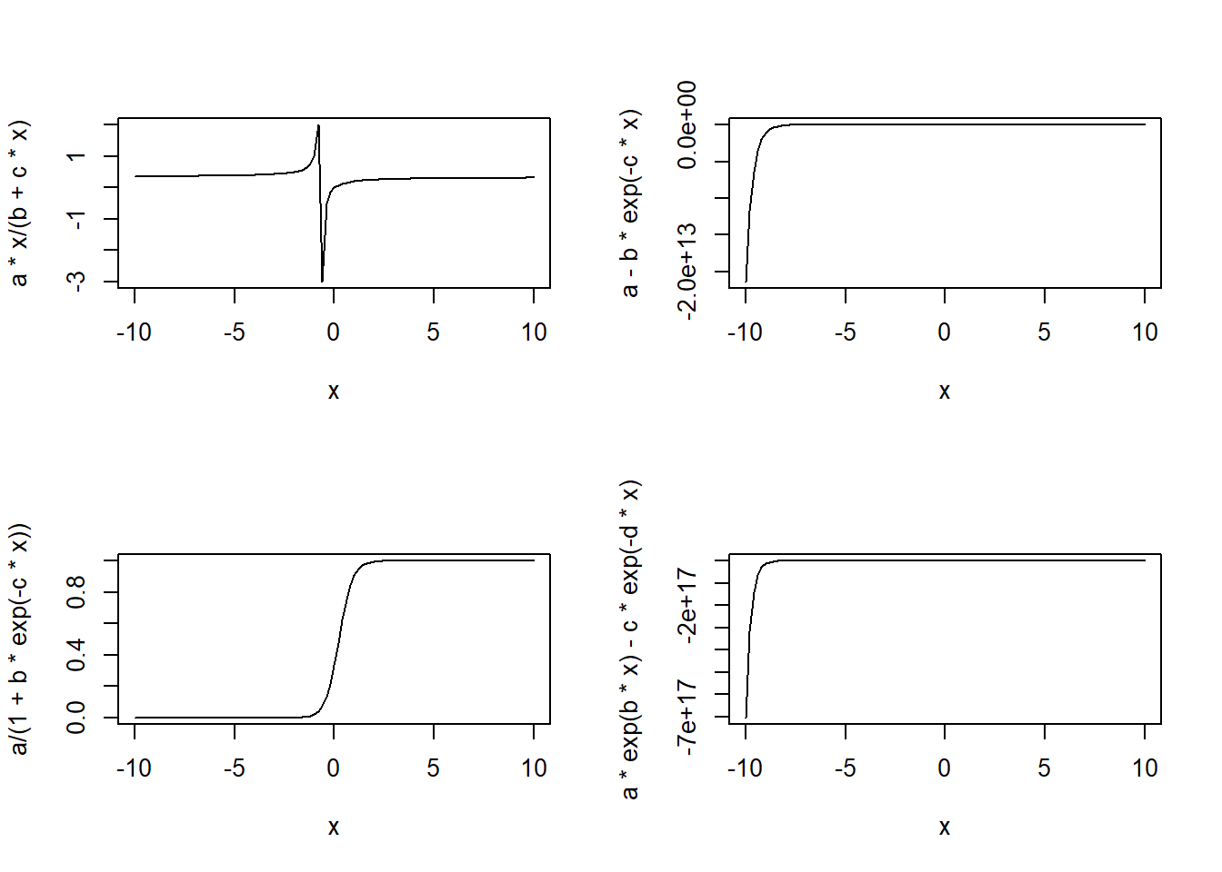
# ggplot() function way
library(ggplot2)
library(gridExtra)
plot1 <- ggplot(data.frame(x = seq(-10, 10, length.out = 100)), aes(x = x)) +
geom_line(aes(y = a * x / (b + c * x))) +
ggtitle("Michaelis-Menten") +
ylab(expression(y == frac(a * x, b + c * x))) +
theme_classic()
plot2 <- ggplot(data.frame(x = seq(-10, 10, length.out = 100)), aes(x = x)) +
geom_line(aes(y = a - b * exp(-c * x))) +
ggtitle("3-parameter asymptotic exponential") +
ylab(expression(y == a - b * e^(-c * x))) +
theme_classic()
plot3 <- ggplot(data.frame(x = seq(-10, 10, length.out = 100)), aes(x = x)) +
geom_line(aes(y = a / (1 + b * exp(-c * x)))) +
ggtitle("3-parameter logistic") +
ylab(expression(y == frac(a, 1 + b * e^(-c * x)))) +
theme_classic()
plot4 <- ggplot(data.frame(x = seq(-10, 10, length.out = 100)), aes(x = x)) +
geom_line(aes(y = a * exp(b * x) - c * exp(-d * x))) +
ggtitle("Biexponential") +
ylab(expression(y == a * e^(b * x) - c * e^(-d * x))) +
theme_classic()
grid.arrange(plot1, plot2, plot3, plot4, ncol = 2)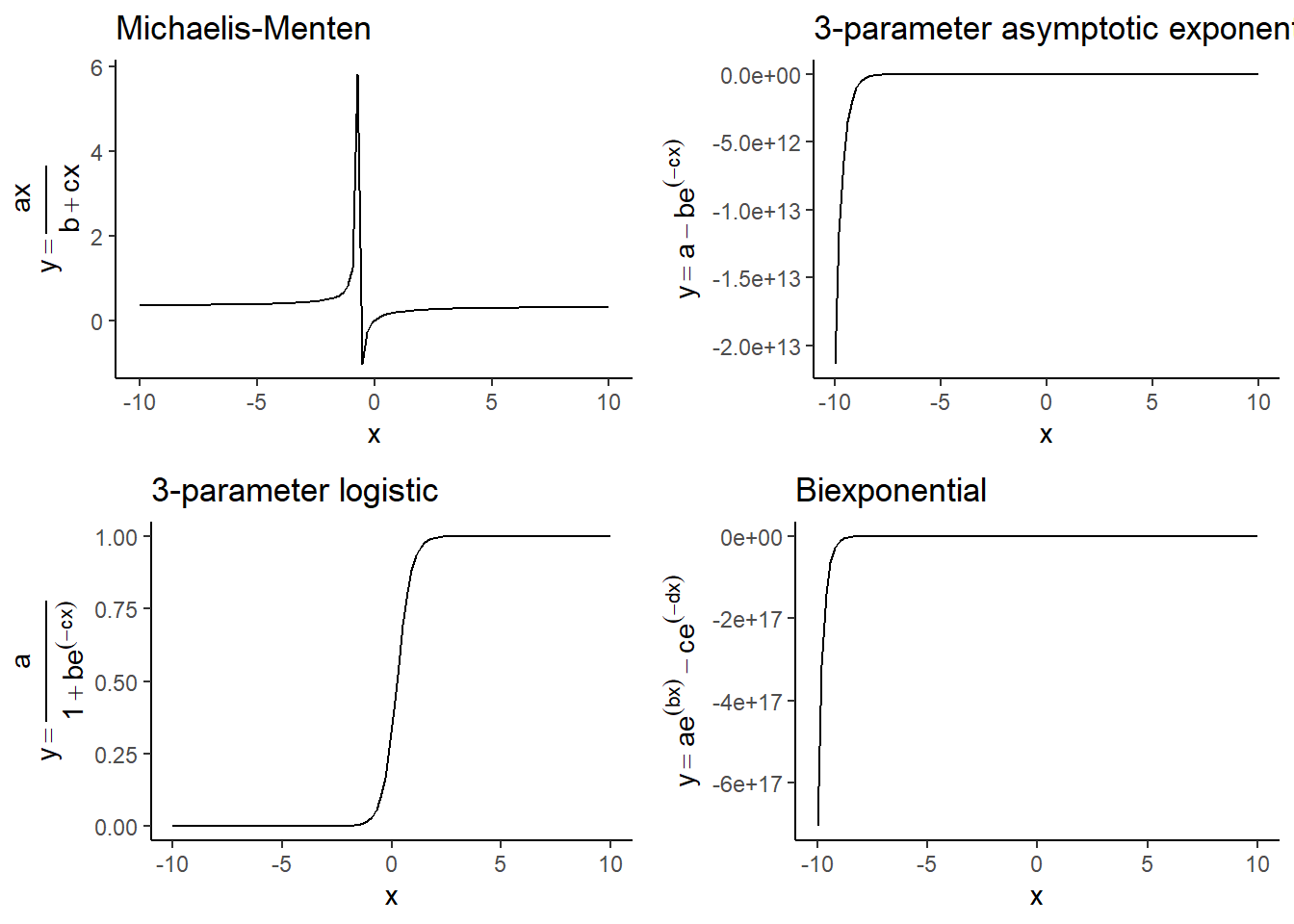
16.1.4 Coefficient
Coefficient of determination (\(R^2\)) formula:
\[R^2=\frac{SSR}{SST}=\frac{\sum_{}^{}(y'-\bar{y})^2}{\sum_{}^{}(y-\bar{y})^2}\]
Pearson Correlation Coefficient (\(r\)) formula:
\[r =\frac{\sum_{i=1}^{n}\left(x_{i}-\bar{x}\right)\left(y_{i}-\bar{y}\right)}{\sqrt{\sum_{i=1}^{n}\left(x_{i}-\bar{x}\right)^{2} \sum_{i=1}^{n}\left(y_{i}-\bar{y}\right)^{2}}}\]
16.1.5 Partial coefficient of determination
For linear regression, \(r^2 = R^2\). But for non-linear regression, because \(SST \neq SSE + SSR\) so \(R^2 \neq r^2\).
Measure the fitting of non-linear regression model. Its definition formula is:
\[R^2=1-\frac{SSE}{SST}\]
16.2 Workflow
16.2.1 Original data
Reaction rate ~ concentration
dtf <- read.table("data/mm.txt", header=T)
library(ggplot2)
ggplot(dtf) + geom_point(aes(conc, rate)) + theme_bw()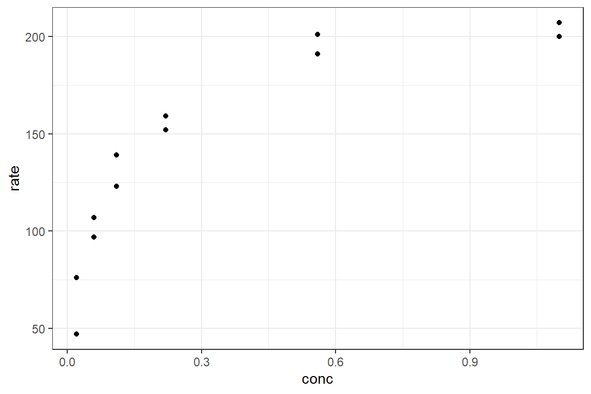
16.2.2 Fit the model manually
Fit Michaelis-Menten model (m1): \(y=\frac{a x}{b+x}\)
Features:
- The curve passes through the origin
- Rising rate of the curve diminishes with the increasing of \(x\)
- Function has an asymptote \(y = a\)
- \(y = \frac{a}{2}\) when \(x = b\)
Fit 3-parameter asymptotic exponential model (m2): \(y=a-b \mathrm{e}^{-c x}\)
m1 <- nls(rate ~ a * conc / (b + conc), data = dtf, start = list(a = 200, b = 0.03))
m2 <- nls(rate ~ a - b * exp(-c * conc), data = dtf, start = list(a = 200, b = 150, c = 5))16.2.3 Automatic way
Find the start value of model parameters is very hard, so here are some automatic functions:
| Function | Model |
|---|---|
SSasymp() |
asymptotic regression model |
SSasympOff() |
asymptotic regression model with an offset |
SSasympOrig() |
asymptotic regression model through the origin |
SSbiexp() |
biexponential model |
SSfol() |
first-order compartment model |
SSfpl() |
four-parameter logistic model |
SSgompertz() |
Gompertz growth model |
SSlogis() |
logistic model |
SSmicmen() |
Michaelis–Menten model |
SSweibull() |
Weibull growth curve model |
m1 <- nls(rate ~ SSmicmen(conc, a, b), data = dtf)
m1Nonlinear regression model
model: rate ~ SSmicmen(conc, a, b)
data: dtf
a b
212.68371 0.06412
residual sum-of-squares: 1195
Number of iterations to convergence: 0
Achieved convergence tolerance: 1.937e-06Result: \(r = \frac{212.7c}{0.06412+c}\)
summary(m1)
Formula: rate ~ SSmicmen(conc, a, b)
Parameters:
Estimate Std. Error t value Pr(>|t|)
a 2.127e+02 6.947e+00 30.615 3.24e-11 ***
b 6.412e-02 8.281e-03 7.743 1.57e-05 ***
---
Signif. codes: 0 '***' 0.001 '**' 0.01 '*' 0.05 '.' 0.1 ' ' 1
Residual standard error: 10.93 on 10 degrees of freedom
Number of iterations to convergence: 0
Achieved convergence tolerance: 1.937e-06m2 <- nls(rate ~ SSasympOff(conc, a, b, c), data = dtf)
m2Nonlinear regression model
model: rate ~ SSasympOff(conc, a, b, c)
data: dtf
a b c
200.94280 1.85368 -0.04298
residual sum-of-squares: 1009
Number of iterations to convergence: 0
Achieved convergence tolerance: 1.768e-06Result: \(r = 201 - 153 e^{-6.38c}\)
summary(m2)
Formula: rate ~ SSasympOff(conc, a, b, c)
Parameters:
Estimate Std. Error t value Pr(>|t|)
a 200.94280 5.97460 33.633 8.95e-11 ***
b 1.85368 0.16218 11.430 1.16e-06 ***
c -0.04298 0.01486 -2.893 0.0178 *
---
Signif. codes: 0 '***' 0.001 '**' 0.01 '*' 0.05 '.' 0.1 ' ' 1
Residual standard error: 10.59 on 9 degrees of freedom
Number of iterations to convergence: 0
Achieved convergence tolerance: 1.768e-0616.2.4 Partial coefficient of determination
Formula: \(R^{2}=1-\frac{SSE}{SST}\)
calc_R2 <- function(model) {
ms <- summary(model)
sse <- as.vector((ms[[3]])^2 * ms$df[2])
null <- lm(dtf$rate ~ 1)
sst <- as.vector(unlist(summary.aov(null)[[1]][2]))
1 - sse/sst
}
c(calc_R2(m1), calc_R2(m2))[1] 0.9612608 0.967298716.2.5 Visualization
xv <- seq(0, 1.2, .01)
y1 <- predict(m1, list(conc = xv))
y2 <- predict(m2, list(conc = xv))
dtf_predicted <- data.frame(xv, y1, y2)
ggplot(dtf) +
geom_point(aes(conc, rate)) +
geom_line(aes(xv, y1, color = 'Michaelis-Menten model'), data = dtf_predicted) +
geom_line(aes(xv, y2, color = '3-parameter asymptotic exponential model'), data = dtf_predicted) +
theme_bw() +
scale_color_manual(values = c('Michaelis-Menten model' = 'blue', '3-parameter asymptotic exponential model' = 'red')) +
labs(color = 'Model') +
guides(color = guide_legend(title = 'Models'))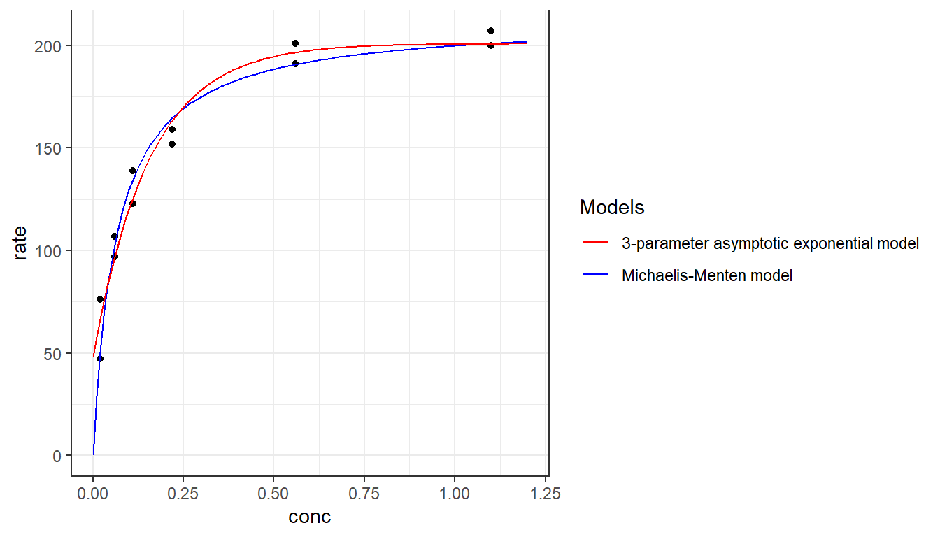
17 Tests for distributions
17.1 Distributions and their R functions
| Distribution | d | p | q | r |
|---|---|---|---|---|
| Beta | pbeta() |
qbeta() |
dbeta() |
rbeta() |
| Binomial | pbinom() |
qbinom() |
dbinom() |
rbinom() |
| Cauchy | pcauchy() |
qcauchy() |
dcauchy() |
rcauchy() |
| Chi-Square | pchisq() |
qchisq() |
dchisq() |
rchisq() |
| Exponential) | pexp() |
qexp() |
dexp() |
rexp() |
| F | pf() |
qf() |
df() |
rf() |
| Gamma | pgamma() |
qgamma() |
dgamma() |
rgamma() |
| Geometric | pgeom() |
qgeom() |
dgeom() |
rgeom() |
| Hyper geometric | phyper() |
qhyper() |
dhyper() |
rhyper() |
| Logistic | plogis() |
qlogis() |
dlogis() |
rlogis() |
| Log Normal | plnorm() |
qlnorm() |
dlnorm() |
rlnorm() |
| Negative Binomial | pnbinom() |
qnbinom() |
dnbinom() |
rnbinom() |
| Normal | pnorm() |
qnorm() |
dnorm() |
rnorm() |
| Poisson | ppois() |
qpois() |
dpois() |
rpois() |
| Student t | pt() |
qt() |
dt() |
rt() |
| Studentized Range | ptukey() |
qtukey() |
dtukey() |
rtukey() |
| Uniform | punif() |
qunif() |
dunif() |
runif() |
| Weibull | pweibull() |
qweibull() |
dweibull() |
rweibull() |
| Wilcoxon Rank Sum Statistic | pwilcox() |
qwilcox() |
dwilcox() |
rwilcox() |
| Wilcoxon Signed Rank Statistic | psignrank() |
qsignrank() |
dsignrank() |
rsignrank() |
Distribution functions in R: prefix + root_name
- d for “density”, the density function (PDF).
- p for “probability”, the cumulative distribution function (CDF).
- q for “quantile” or “critical”, the inverse of CDF.
- r for “random”, a random variable having the specified distribution
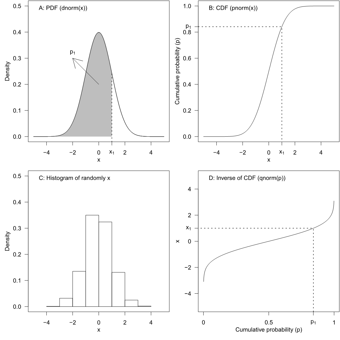
Some common distribution:
| Distribution | Parameters | Expression | Mean | Variance |
|---|---|---|---|---|
| Bernoulli trial | \(p\) | \(q\) | \(p\) | \(pq\) |
| Binomial | \(n, p\) | \(C(n, x) p^x q^{n-x}\) | \(np\) | \(npq\) |
| Poisson | \(\lambda\) | \(e^{-\lambda} \lambda^x / x !\) | \(\lambda\) | \(\lambda\) |
| Normal | \(\mu, \sigma\) | \(\frac{1}{\sqrt{2 \pi \sigma}} e^{-(x-\mu)^2 / 2 \sigma^2}\) | \(\mu\) | \(\sigma^2\) |
| Std. Normal | \(z\) | \(\frac{1}{\sqrt{2 \pi}} e^{-z^2 / 2}\) | \(0\) | \(1\) |
| Student-t | \(v\) | \(\frac{\Gamma\left(\frac{v+1}{2}\right)}{\sqrt{v \pi} \Gamma\left(\frac{v}{2}\right)}\left(1+\frac{x^2}{v}\right)^{-\frac{v+1}{2}}\) | \(0\) | \(\left\{\begin{array}{cc}v /(v-2) & \text { for } v>2 \\ \infty & \text { for } 1<v \leq 2 \\ \text { undefined } & \text { otherwise }\end{array}\right.\) |
17.2 Empirical distribution function (EDF or eCDF)
17.2.1 Concepts
\[F_{n}(x)= \begin{cases}0, & \text { for } x<y_{1} \\ k / n, & \text { for } y_{k} \leqslant x<y_{k+1}\qquad (k=1,2, \ldots, n-1) \\ 1, & \text { for } x \geqslant y_{n}\end{cases}\]
Empirical distribution function (EDF) is a way of representing the cumulative distribution function (CDF) of a set of data. The EDF is calculated by ordering the data from smallest to largest, and then assigning a probability to each data point based on its rank in the distribution.
Specifically, the EDF assigns a probability of 1/n to each of the n data points, where n is the sample size. Then, the EDF at any given point x is the proportion of data points that are less than or equal to x.
17.2.2 Visualization
code
par(mfrow = c(2, 2))
x1 <- rnorm(10)
x2 <- rnorm(20)
x3 <- rnorm(50)
x4 <- rnorm(100)
plot(ecdf(x1))
curve(pnorm, col = 'red', add = TRUE)
plot(ecdf(x2))
curve(pnorm, col = 'red', add = TRUE)
plot(ecdf(x3))
curve(pnorm, col = 'red', add = TRUE)
plot(ecdf(x4))
curve(pnorm, col = 'red', add = TRUE)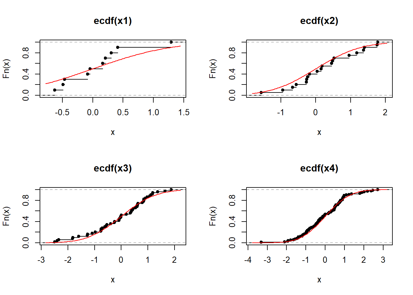
17.3 Kolmogorov-Smirnov test
17.3.1 Concepts
The KS test works by comparing the maximum distance between the EDF and the CDF, called the KS statistic, to a critical value calculated from the null distribution of the test statistic. If the calculated KS statistic is larger than the critical value, the null hypothesis that the sample is drawn from the theoretical distribution is rejected.
critical values for D for one sample (\(n\le40\)):
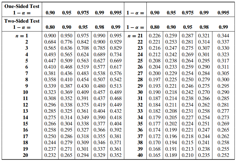
Asymptotic critical values for \(D\) for one sample (small sample sizes):
| \(\alpha\) | 0.2 | 0.1 | 0.05 | 0.02 | 0.01 |
|---|---|---|---|---|---|
| Critical \(D\) | \(1.07\sqrt{\frac{1}{n}}\) | \(1.14\cdot\sqrt{\frac{1}{n}}\) | \(1.22\cdot\sqrt{\frac{1}{n}}\) | \(1.52\cdot\sqrt{\frac{1}{n}}\) | \(1.63 \cdot\sqrt{\frac{1}{n}}\) |
critical values for D for two sample (\(n\le40\)):

Asymptotic critical values for \(D\) for one sample (large samle sizes):
| \(\alpha\) | 0.2 | 0.1 | 0.05 | 0.02 | 0.01 |
|---|---|---|---|---|---|
| Critical \(D\) | \(1.07\sqrt{\frac{m+n}{n}}\) | \(1.14\cdot\sqrt{\frac{m+n}{n}}\) | \(1.22\cdot\sqrt{\frac{m+n}{n}}\) | \(1.52\cdot\sqrt{\frac{m+n}{n}}\) | \(1.63 \cdot\sqrt{\frac{m+n}{n}}\) |
17.3.2 Visualization
code
# package ‘kolmin’ is not available for this version of R
library(kolmim)
pvalue <- pkolm(d = 0.1, n = 30)
nks <- c(10, 20, 30, 50, 80, 100)
x <- seq(0.01, 1, 0.01)
y <- sapply(x, pkolm, n = nks[1])
plot(x, y, type = 'l', las = 1, xlab = 'D', ylab = 'CDF')
for (i in 2:length(nks)) lines(x, sapply(x, pkolm, n = nks[i]), col = i)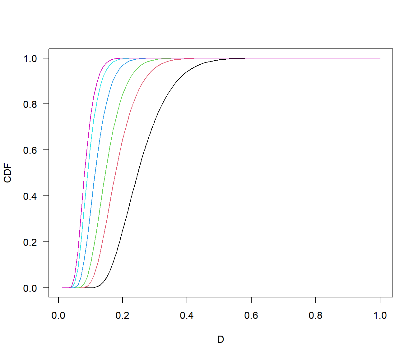
17.3.3 One-sample test
Hypothesis:
\(H_{0}: F(x)=F_{0}(x)\) The CDF of x is a given reference distribution function \(F_0(x)\).
Test statistic:
\(D_{n}=\sup _{x}\left[\left|F_{n}(x)-F_{0}(x)\right|\right]\)
\(D_{n}\): the supremum distance between the empirical distribution function of given sample and the cumulative distribution function of the given reference distribution.
Example:
# Original dataset
x0 <- c(108, 112, 117, 130, 111, 131, 113, 113, 105, 128)
x0_mean <- mean(x0)
x0_sd <- sd(x0)
eCDF <- ecdf(x0)
# cumulative distribution function F(x) of the reference distribution
CDF <- pnorm(x0, x0_mean, x0_sd)
# create a data frame to put values into
df <- data.frame(data = x0, eCDF = eCDF(x0), CDF = CDF)
# visualization
library(ggplot2)
ggplot(df, aes(data)) +
stat_ecdf(size=1,aes(colour = "Empirical CDF (Fn(x))")) +
stat_function(fun = pnorm, args = list(x0_mean, x0_sd), aes(colour = "Theoretical CDF (F(x))")) +
xlab("Sample data") +
ylab("Cumulative probability") +
scale_y_continuous(breaks=seq(0, 1, by = 0.2))+
theme(legend.title=element_blank())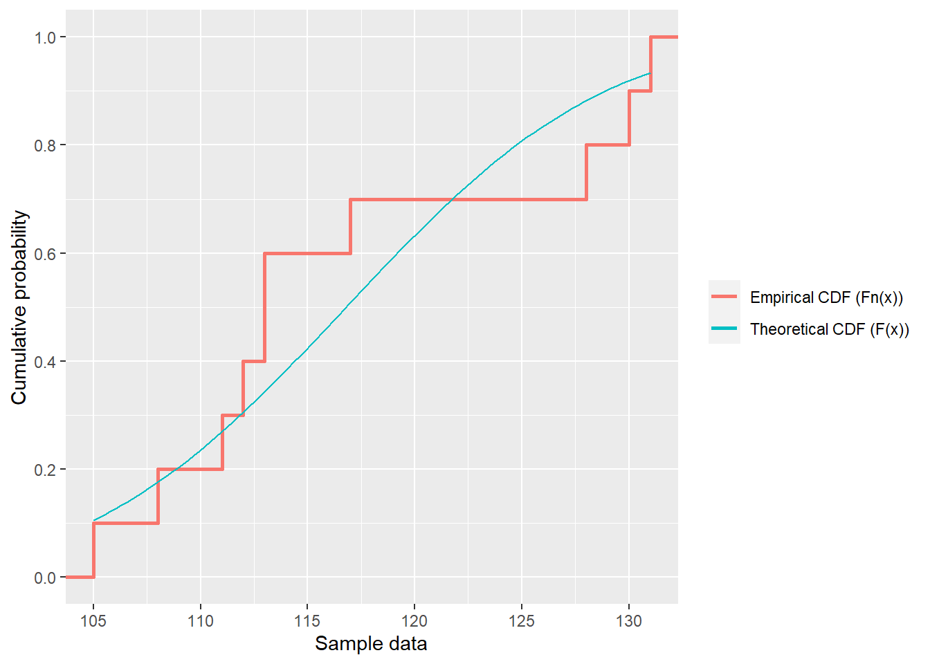
# sort values of sample observations and remove duplicates
x <- unique(sort(x0))
# Calculate D
Daft <- abs(eCDF(x) - pnorm(x, x0_mean, x0_sd))
Daft[1] 0.005874162 0.024147672 0.030327372 0.094264640 0.256212096 0.191556764
[7] 0.082045735 0.018782968 0.066450468Dbef <- abs(c(0, eCDF(x)[-length(x)]) - pnorm(x, x0_mean, x0_sd))
Dbef[1] 0.10587416 0.07585233 0.06967263 0.00573536 0.05621210 0.09155676 0.18204573
[8] 0.11878297 0.03354953D_score <- max(c(Daft, Dbef))
D_score[1] 0.2562121One step in R:
ks.test(x0,'pnorm', x0_mean, x0_sd)
Asymptotic one-sample Kolmogorov-Smirnov test
data: x0
D = 0.25621, p-value = 0.5276
alternative hypothesis: two-sidedDecision:
We cannot reject \(H_0\) that the data are normally distributed at \(\alpha = 0.05\).
Conclusion:
The data follows a normal distribution.
17.3.4 Two-sample test
Hypothesis:
\(H_0\): Two populations follow a common probability distribution.
Test statistic:
\(D_{n,m}=\sup _{x}\left[\left|F_{1, n}(x)-F_{2, m}(x)\right|\right]\)
Example:
# Original dataset
sample1 <- c(165, 168, 172, 177, 180, 182)
sample2 <- c(163, 167, 169, 175, 175, 179, 183, 185)
mean1 <- mean(sample1)
mean2 <- mean(sample2)
sd1 <- sd(sample1)
sd2 <- sd(sample2)
# empirical distribution function Fn(x)
eCDF1 <- ecdf(sample1)
eCDF1(sample1)[1] 0.1666667 0.3333333 0.5000000 0.6666667 0.8333333 1.0000000# empirical distribution function Fm(x)
eCDF2 <- ecdf(sample2)
eCDF2(sample2)[1] 0.125 0.250 0.375 0.625 0.625 0.750 0.875 1.000# visualization
group2 <- c(rep("sample1", length(sample1)), rep("sample2", length(sample2)))
df2 <- data.frame(all = c(sample1,sample2), group = group2)
library(ggplot2)
ggplot(df2, aes(x = all, group = group, color = group2)) +
stat_ecdf(size=1) +
xlab("Sample data") +
ylab("Cumulative probability") +
theme(legend.title=element_blank())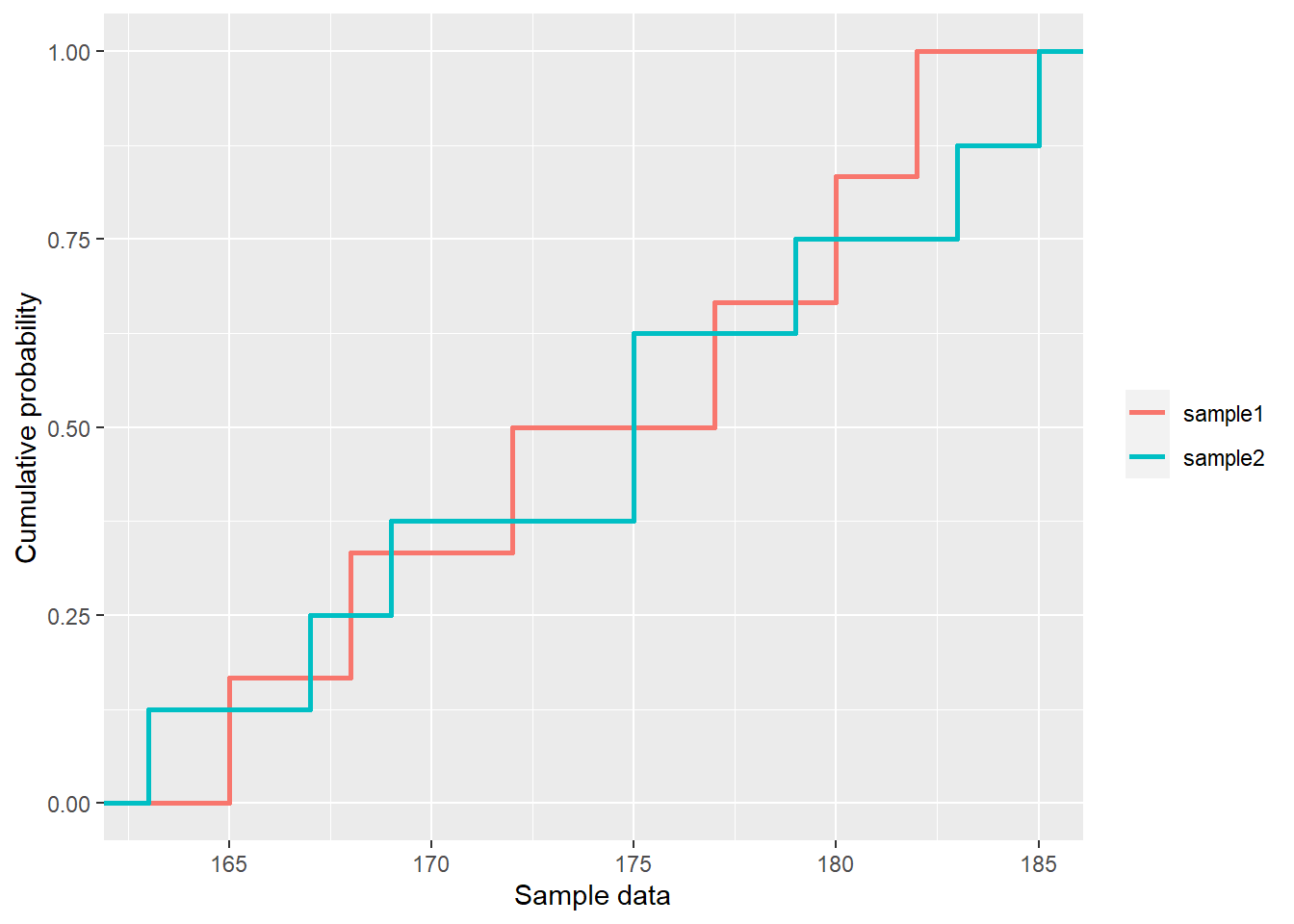
# merge, sort observations of two samples, and remove duplicates
x2 <- unique(sort(c(sample1,sample2)))
# calculate D and its location
D2 <- max(abs(eCDF1(x2) - eCDF2(x2)))
idxD2 <- which.max(abs(eCDF1(x2) - eCDF2(x2))) # the index of x-axis value
xD2 <- x2[idxD2] # corresponding x-axis value
D2[1] 0.25One step in R:
ks.test(sample1, sample2)
Exact two-sample Kolmogorov-Smirnov test
data: sample1 and sample2
D = 0.25, p-value = 0.9281
alternative hypothesis: two-sidedDecision:
We cannot reject the \(H_0\) at \(\alpha = 0.05\).
Test statistic:
We can conclude that sample 1 and sample 2 come from the same distributions.
18 Principal component analysis
18.1 Concepts
18.1.1 Defination
A dimensionality reduction technique that enables identification of correlations and patterns in a data set so that it can be transformed into a data set of significantly lower dimension without loss of any important information.
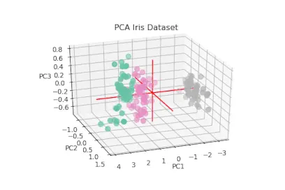
18.1.2 Procedure
Move the center of the coordinate axis to the center of the data, and then rotate the coordinate axis to maximize the variance of the data projected on the C1 axis. C1 is called “the first principal component”. That is, the projection of all the data in this direction is the most scattered.
Find an axis (C2), so that the covariance (correlation coefficient) between C2 and C1 is 0, so as to avoid overlapping with C1 information. Make the variance of data in this direction as large as possible. C2 is called “the second principal component”.
Similarly, find the third principal component, the fourth principal component… The \(n_{th}\) principal component. \(n\) random variables can have n principal components.
18.1.3 Usages in R
Two functions:
prcomp()princomp()
Example:
com1 <- prcomp(iris[,1:4], center = TRUE, scale. = TRUE)
summary(com1)Importance of components:
PC1 PC2 PC3 PC4
Standard deviation 1.7084 0.9560 0.38309 0.14393
Proportion of Variance 0.7296 0.2285 0.03669 0.00518
Cumulative Proportion 0.7296 0.9581 0.99482 1.00000dt <- as.matrix(scale(iris[, 1:4])) # First need to do normalization
com2 <- princomp(dt, cor = T)
summary(com2)Importance of components:
Comp.1 Comp.2 Comp.3 Comp.4
Standard deviation 1.7083611 0.9560494 0.38308860 0.143926497
Proportion of Variance 0.7296245 0.2285076 0.03668922 0.005178709
Cumulative Proportion 0.7296245 0.9581321 0.99482129 1.000000000Warning: only applies to matrices with more rows than columns.
18.2 Data transformation
| Normalization | Standardization |
|---|---|
| \(x_{norm} = \frac{x -x_{min}}{x_{max} - x_{min}}\) | \(z = \frac{x-\mu}{\sigma}\) |
| Minimum and maximum value of features are used for scaling | Mean and standard deviation is used for scaling |
| When features are of different scales | When we want to ensure zero mean and unit standard deviation |
| 0~1 | Not bounded to a certain range. |
| Much affected by outliers | Less affected by outliers |
| It is useful when we don’t know about the distribution | It is useful when the feature distribution is Normal or Gaussian |
18.3 Workflow
18.3.1 Data preprocess
# Iris example
dt <- as.matrix(scale(iris[, 1:4]))
head(dt, 4) Sepal.Length Sepal.Width Petal.Length Petal.Width
[1,] -0.8976739 1.01560199 -1.335752 -1.311052
[2,] -1.1392005 -0.13153881 -1.335752 -1.311052
[3,] -1.3807271 0.32731751 -1.392399 -1.311052
[4,] -1.5014904 0.09788935 -1.279104 -1.31105218.3.2 Correlation coefficient (covariance) matrix
rm1 <- cor(dt)
rm1 Sepal.Length Sepal.Width Petal.Length Petal.Width
Sepal.Length 1.0000000 -0.1175698 0.8717538 0.8179411
Sepal.Width -0.1175698 1.0000000 -0.4284401 -0.3661259
Petal.Length 0.8717538 -0.4284401 1.0000000 0.9628654
Petal.Width 0.8179411 -0.3661259 0.9628654 1.000000018.3.3 Eigenvalues and eigenvectors
rs1 <- eigen(rm1)
# Extract the eigenvalue in the result, that is the variance of each principal component
val <- rs1$values
# Convert to standard deviation
Standard_deviation <- sqrt(val)
# Calculate variance contribution rate and cumulative contribution rate
Proportion_of_Variance <- val / sum(val)
Cumulative_Proportion <- cumsum(Proportion_of_Variance)
# Draw scree plot
plot(val, type = "b", las = 1,
xlab = "Principal component number", ylab = "Principal component variance")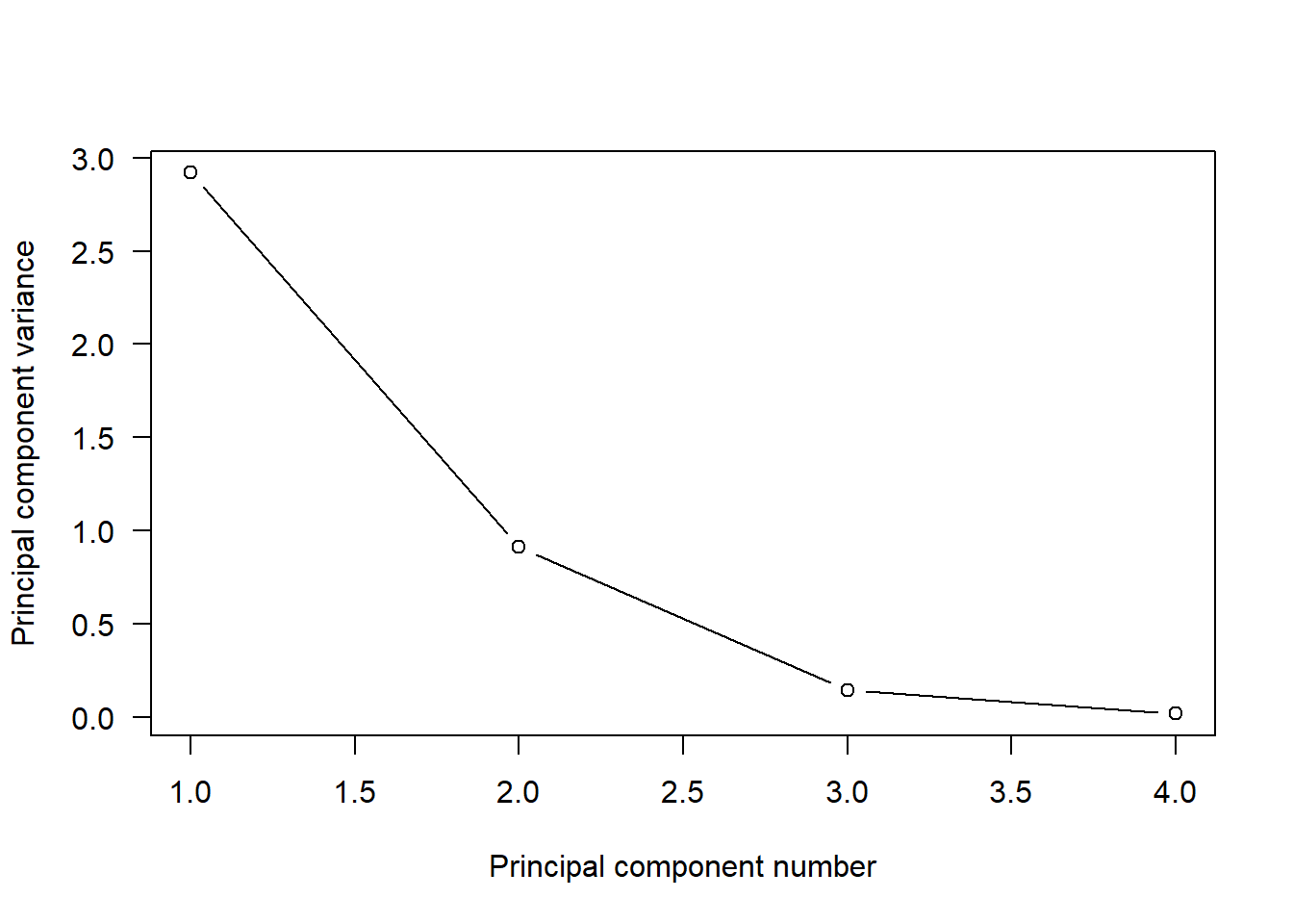
Then choose the right principal component number
18.3.4 Principal component score
# Feature vectors in extraction results
U <- as.matrix(rs1$vectors)
# Perform matrix multiplication to obtain PC score
PC <- dt %*% U
colnames(PC) <- c("PC1","PC2","PC3","PC4")
df <- data.frame(PC, iris$Species)
head(df, 4) PC1 PC2 PC3 PC4 iris.Species
1 -2.257141 -0.4784238 0.1272796 0.02408751 setosa
2 -2.074013 0.6718827 0.2338255 0.10266284 setosa
3 -2.356335 0.3407664 -0.0440539 0.02828231 setosa
4 -2.291707 0.5953999 -0.0909853 -0.06573534 setosa18.3.5 One step way
com <- prcomp(iris[, 1:4], center = TRUE, scale. = TRUE)
df <- data.frame(com$x, iris$Species)18.3.6 Visualization
Draw the main component dispersion point diagram:
library(ggplot2)
# Extract the variance contribution rate of the principal component and generate the coordinate axis title
xlab <- paste0("PC1 (", round(Proportion_of_Variance[1] * 100, 2), "%)")
ylab <- paste0("PC2 (", round(Proportion_of_Variance[2] * 100, 2), "%)")
# Draw a scatter plot and add a confidence ellipse
ggplot(data = df, aes(x = PC1, y = PC2, color = iris.Species)) +
geom_point() + labs(x = xlab, y = ylab) +
stat_ellipse(
aes(fill = iris.Species),
type = "norm",
geom = "polygon",
alpha = 0.2,
color = NA
)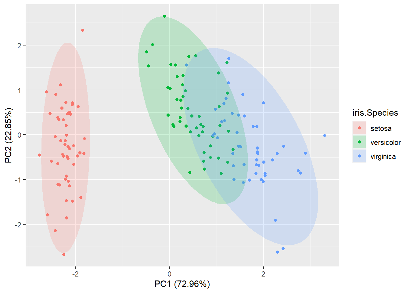
19 Cluster analysis
19.1 Concepts
19.1.1 Definition
Cluster analysis/Clustering: A simple and intuitive method of data simplification. It splits a number of observations or measured variables into groups that are similar in their characteristics or behaviors.
Cluster: A group of objects such that the objects in the cluster are closer (more similar) to the ‘centre’ of their cluster than to the centre of any other cluster. The centre of a cluster is usually the centroid, the average of all the points in the cluster, or the most ‘representative’ point in the cluster.
19.1.2 K-means
Centroid models: Iterative clustering algorithms. Iteratively correct the centroid positions of the clusters and adjust the classification of each data point.
K-mean: Classify a given data set by a certain number (K) of predefined clusters. The most common centroid-based clustering algorithm. Find the partition of the n individuals into k groups that minimises the within-group sum of squares over all variables.
Steps:
- Specify the number of clusters k.
- Assign points to clusters randomly.
- Find the centroids of each cluster.
- Re-assign points according to their closest centroid.
- Re-adjust the positions of the cluster centroids.
- Repeat steps 4 and 5 until no further changes are there.
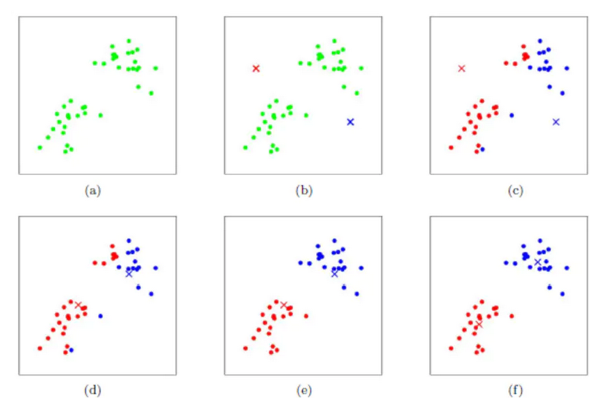
Advantages:
- The fastest centroid-based algorithm.
- Work for large data sets.
- Reduce intra-cluster variance
Disadvantages:
- Performance is affected when there is more noise in the data.
- Outliers can never be studied.
- Even though it reduces intra-cluster variance, it can’t affect or deal with the global minimum variance of measure.
- Very sensitive at clustering data sets of non-convex shaped clusters.
Here is the number of possible partitions depending on the sample size n and number of clusters k. It would be impossible to make a complete enumeration of every possible partition, even with the fastest computers.
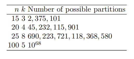
19.1.3 Hierarchical cluster analysis (HCA)
HCA:
Suitable for clustering of small data sets because of the cost on time and space.
Approaches:
Agglomerative (AGNES): Begin with each observation in a distinct (singleton) cluster, and successively merges clusters together until a stopping criterion is satisfied. Bottom-up.
Divisive (DIANA): Begin with all patterns in a single cluster and performs splitting until a stopping criterion is met. Top-down.
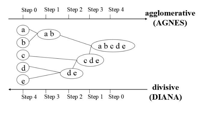
Advantages:
- The similarity of distance and rules is easy to define and less restrictive.
- There is not required to specify the clustering number in advance.
- It can discover the hierarchy of clusters, showing by the tree.
Disadvantages:
- The algorithm is complex.
- It does not scale well, because of the difficulty of choosing merging or splitting points.
19.2 Workflow
19.2.1 Data preprocess
- Same unit —- because of the ignoring of physical meanings, focusing on number.
- Same dimension —- because of the measuring of distance.
newIris <- iris[1:4]
head(newIris, 4) Sepal.Length Sepal.Width Petal.Length Petal.Width
1 5.1 3.5 1.4 0.2
2 4.9 3.0 1.4 0.2
3 4.7 3.2 1.3 0.2
4 4.6 3.1 1.5 0.219.2.2 K-means
Compare the Total Within Sum of Square under different k values, then determine the optimal clustering number:
library(factoextra)
fviz_nbclust(newIris, kmeans, method = "wss")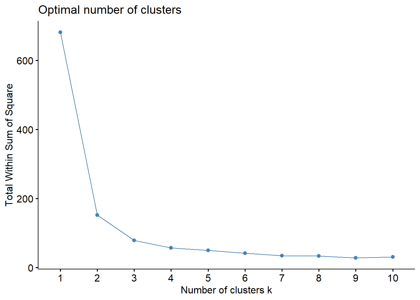
Set k = 3, clustering:
kc <- kmeans(newIris, 3) Create a cross tabulation of clustering and original species to Check the results:
table(iris$Species,kc$cluster)
1 2 3
setosa 17 33 0
versicolor 4 0 46
virginica 0 0 50Visualization:
par(mfrow = c(1, 2))
plot(newIris[c("Sepal.Length", "Sepal.Width")],
col = kc$cluster,
pch = as.integer(iris$Species))
points(kc$centers,
col = 1:3,
pch = 16,
cex = 2)
plot(newIris[c("Petal.Length", "Petal.Width")],
col = kc$cluster,
pch = as.integer(iris$Species))
points(kc$centers,
col = 1:3,
pch = 16,
cex = 2)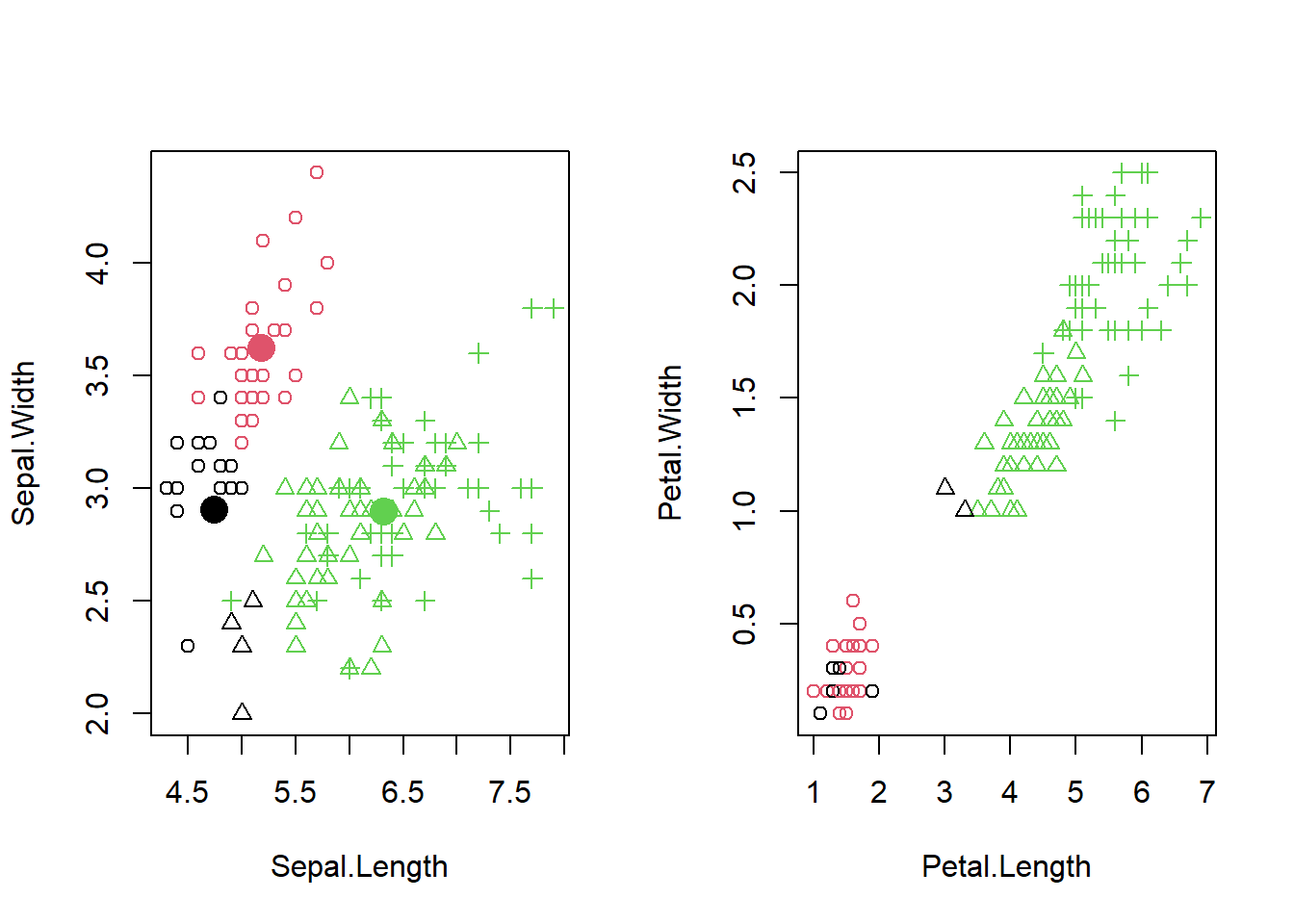
19.2.3 Hierarchical cluster analysis
Box-Cox transformation:explain
A flexible data normalization method which can minimize the skewness. More suitable for the (applied geochemical and) general environmental data. The data for Box-Cox transformation is required to be positive and continuous variables.19.2.3.1 First 3 colomns iris dataset
iris3R <- as.matrix(iris[2:4, -5])
row.names(iris3R) <- c("Object1", "Object2", "Object3")
library(forecast)
iris.transformed <- BoxCox(iris3R, lambda = "auto")
iris.transformed Sepal.Length Sepal.Width Petal.Length Petal.Width
Object1 3.725276 1.941234 0.3967354 -0.8225575
Object2 3.539252 2.131053 0.2981108 -0.8225575
Object3 3.446104 2.036214 0.4950348 -0.8225575
attr(,"lambda")
[1] 0.953813919.2.3.2 euclidean method
Default using “euclidean” for distance measure if not choose methods. Euclidean is a good choice when using low-dimensional data, but usually, it need to normalize the data before.
# calculate the distance matrix
distE <- dist(as.matrix(iris.transformed), method = "euclidean")
distE Object1 Object2
Object2 0.2834833
Object3 0.3108387 0.2375921The distance between Object2 and Object3 is minimum.
Perform HCA (AGNES):
hc1 <- hclust(distE, method = "complete")
# default using "complete"(-linkage) as linkage method if not choose methods
# Draw the dendrogram(Because the cluster solutions grow tree-like)
plot(hc1)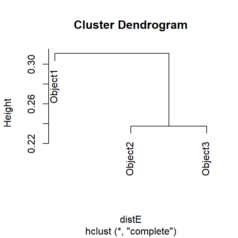
Result: Object2 and Object3 are more similar, and Object1 is more different.
19.2.3.3 canberra method
But if change the distance measure to “canberra”, the situation will be slightly different:
distC <- dist(as.matrix(iris.transformed), method = "canberra")
distC Object1 Object2
Object2 0.2141568
Object3 0.1730378 0.2843751hc2 <- hclust(distC, method = "complete")
plot(hc2)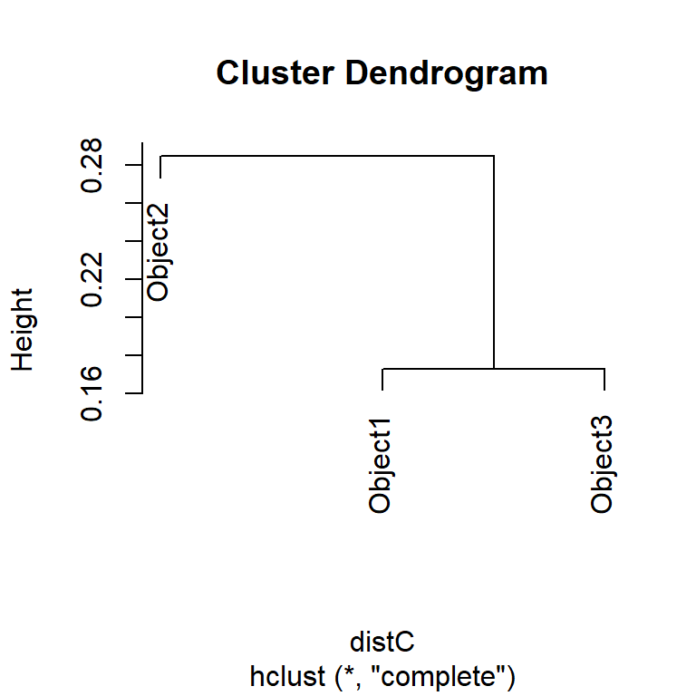
19.2.3.4 Decision
Use agglomerative coefficients (AC, for AGNES) and divisive coefficient (DC, for DIANA) to compare the strength of the hierarchical clustering structures. The stronger the clustering structure, the higher the coefficient (closer to 1).
library(cluster)
# help("coef.hclust")
coef.hclust(hc1)[1] 0.1570945coef.hclust(hc2)[1] 0.2610104Result: As “canberra” has a higher AC, it is stronger.
19.2.3.5 Whole iris dataset clustering
library(cluster)
library(forecast)
iris.trans <- BoxCox(as.matrix(iris[,-5]), lambda = "auto")Perform AGNES:
irisHcA <- agnes(iris.trans, metric = "euclidean", method = "average") # The default setting `metric = "euclidean"`
# Cut the AGNES tree at cluster number(k) = 3
hclusterA <- cutree(irisHcA, k = 3)
tb1 <- table(true = iris$Species, cluster = hclusterA)
tb1 cluster
true 1 2 3
setosa 50 0 0
versicolor 0 46 4
virginica 0 50 0# Extract the agglomerative coefficient. When using agnes/diana(), it's automatically calculated
irisHcA$ac # k-value will not affect the agglomerative coefficients[1] 0.9378719irisHcS <- agnes(iris.trans, method = "single")
hclusterS <- cutree(irisHcS, k = 3)
tb2 <- table(true = iris$Species, cluster = hclusterS)
tb2 cluster
true 1 2 3
setosa 49 1 0
versicolor 0 0 50
virginica 0 0 50irisHcS$ac[1] 0.8807232Perform DIANA:
irisHcD <- diana(iris.trans) # No linkage method, default setting
# Cut at k = 3
hclusterD <- cutree(irisHcD, k = 3)
tb3 <- table(true = iris$Species, cluster = hclusterD)
tb3 cluster
true 1 2 3
setosa 50 0 0
versicolor 0 46 4
virginica 0 3 47# Extract divisive coefficient
irisHcD$dc[1] 0.9555297Result: The no linkage method is better than the average method and the single method in this model.
SessionInfo:
R version 4.2.3 (2023-03-15 ucrt)
Platform: x86_64-w64-mingw32/x64 (64-bit)
Running under: Windows 10 x64 (build 19044)
Matrix products: default
locale:
[1] LC_COLLATE=Chinese (Simplified)_China.utf8
[2] LC_CTYPE=Chinese (Simplified)_China.utf8
[3] LC_MONETARY=Chinese (Simplified)_China.utf8
[4] LC_NUMERIC=C
[5] LC_TIME=en_GB.UTF-8
attached base packages:
[1] stats graphics grDevices utils datasets methods base
other attached packages:
[1] cluster_2.1.4 forecast_8.21 factoextra_1.0.7 gridExtra_2.3
[5] qcc_2.7 faraway_1.0.8 nnet_7.3-18 jmv_2.3.4
[9] car_3.1-2 carData_3.0-5 ISLR_1.4 biotools_4.2
[13] mvnormalTest_1.0.0 rstatix_0.7.2 MASS_7.3-58.2 gplots_3.1.3
[17] agricolae_1.3-5 openair_2.16-0 lubridate_1.9.2 forcats_1.0.0
[21] stringr_1.5.0 dplyr_1.1.0 purrr_1.0.1 readr_2.1.4
[25] tibble_3.2.1 tidyverse_2.0.0 latex2exp_0.9.6 patchwork_1.1.2
[29] ggplot2_3.4.2 Epi_2.47 tidyr_1.3.0 magrittr_2.0.3
[33] knitr_1.42
loaded via a namespace (and not attached):
[1] backports_1.4.1 copula_1.1-2 corrplot_0.92
[4] plyr_1.8.8 splines_4.2.3 pspline_1.0-19
[7] listenv_0.9.0 AlgDesign_1.2.1 equatiomatic_0.3.1
[10] digest_0.6.31 foreach_1.5.2 htmltools_0.5.4
[13] fansi_1.0.3 tzdb_0.3.0 etm_1.1.1
[16] globals_0.16.2 recipes_1.0.5 gower_1.0.1
[19] stabledist_0.7-1 xts_0.13.1 hardhat_1.3.0
[22] timechange_0.2.0 tseries_0.10-54 jpeg_0.1-10
[25] colorspace_2.1-0 ggrepel_0.9.3 haven_2.5.2
[28] xfun_0.37 jsonlite_1.8.4 hexbin_1.28.3
[31] lme4_1.1-31 survival_3.5-3 zoo_1.8-11
[34] iterators_1.0.14 glue_1.6.2 gtable_0.3.3
[37] ipred_0.9-14 questionr_0.7.8 future.apply_1.10.0
[40] quantmod_0.4.22 maps_3.4.1 abind_1.4-5
[43] scales_1.2.1 pscl_1.5.5 mvtnorm_1.1-3
[46] GGally_2.1.2 mvnormtest_0.1-9 miniUI_0.1.1.1
[49] Rcpp_1.0.10 xtable_1.8-4 cmprsk_2.2-11
[52] mapproj_1.2.11 lava_1.7.2.1 prodlim_2023.03.31
[55] stats4_4.2.3 htmlwidgets_1.6.2 RColorBrewer_1.1-3
[58] ellipsis_0.3.2 pkgconfig_2.0.3 reshape_0.8.9
[61] farver_2.1.1 deldir_1.0-6 utf8_1.2.3
[64] caret_6.0-94 reshape2_1.4.4 tidyselect_1.2.0
[67] labeling_0.4.2 rlang_1.1.0 later_1.3.0
[70] munsell_0.5.0 tools_4.2.3 cli_3.6.1
[73] jmvcore_2.3.19 generics_0.1.3 moments_0.14.1
[76] broom_1.0.4 evaluate_0.20 fastmap_1.1.0
[79] yaml_2.3.7 ModelMetrics_1.2.2.2 caTools_1.18.2
[82] future_1.32.0 nlme_3.1-162 mime_0.12
[85] compiler_4.2.3 rstudioapi_0.14 curl_5.0.0
[88] png_0.1-8 ggsignif_0.6.4 klaR_1.7-2
[91] pcaPP_2.0-3 stringi_1.7.12 gsl_2.1-8
[94] highr_0.10 stargazer_5.2.3 lattice_0.20-45
[97] Matrix_1.5-3 nloptr_2.0.3 urca_1.3-3
[100] vctrs_0.6.2 pillar_1.9.0 lifecycle_1.0.3
[103] ADGofTest_0.3 lmtest_0.9-40 combinat_0.0-8
[106] data.table_1.14.8 bitops_1.0-7 httpuv_1.6.9
[109] R6_2.5.1 latticeExtra_0.6-30 promises_1.2.0.1
[112] KernSmooth_2.23-20 parallelly_1.35.0 codetools_0.2-19
[115] boot_1.3-28.1 gtools_3.9.4 withr_2.5.0
[118] nortest_1.0-4 fracdiff_1.5-2 mgcv_1.8-42
[121] parallel_4.2.3 hms_1.1.3 quadprog_1.5-8
[124] rpart_4.1.19 grid_4.2.3 labelled_2.11.0
[127] timeDate_4022.108 class_7.3-21 minqa_1.2.5
[130] rmarkdown_2.21 TTR_0.24.3 ggpubr_0.6.0
[133] pROC_1.18.0 numDeriv_2016.8-1.1 shiny_1.7.4
[136] base64enc_0.1-3 interp_1.1-4